Contents
1 Create your first graph: We will draw a parabola f(x) = (x-5)**2 | |
| step 1.1 | Start the program. |
| step 1.2 | From the File menu (it is the only available right now), choose new. |
| step 1.3 | In the "Select File Type" dialogue window, choose "spreadsheet" and push "OK". A blank spreadsheet "document1" is created. |
| step 1.4 | Click in the spreadsheet cell at column 1, row 1. |
| Then type (without the quote marks): "mV" followed by <RETURN>, then type "0" <RETURN>, "1" <RETURN> etc. until "10" <RETURN>. If you type a wrong character, use the <BACKSPACE> key. | |
| step 1.5 | Click in the spreadsheet cell at column 2, row 1. |
| Then type (without the quote marks): "mA" followed by <RETURN>, then type "25" , "16" , "9" , "4" , "1" , "0" , "1" , "4" , "9" , "16" , "25", where each number is followed by a <RETURN> | |
The spreadsheet should now look like: | |
| step 1.6 | Click on "column" key number 1 and, while keeping the left mouse button depressed, move onto column key 2 and release the mouse button. Now the two columns 1 & 2 are selected: |
| step 1.7 | From the Modify/Stats menu select Line Plot. |
| step 1.8 | In the "Set Columns" dialogue window check "X". This means that column 1 will furnish the X-coordinate. |
| step 1.9 | Advance one column by pushing the |
| step 1.10 | Push the "OK" button. A new drawing window "document2" is created containing the graph: |
| step 1.11 | From the File menu choose save (document2 needs to be the active window. If you have clicked on document1, reactivate document2 by clicking on its title bar before going to the File menu). In the "Save" dialogue window type "step1" as filename. The title bar now reads "step1.his" (the extension is added automatically). |
| Note that the column keys 1 & 2 in the spreadsheet now contain a "°" character. This means that these columns are linked with a graph on a drawing sheet. The use of these links is the subject of the next exercise. | |
2 Edit the graph using the spreadsheet | |
| If you just carried out step 1, leave the program and restart it. (It is not necessary to save document1). | |
| step 2.1 | From the File menu choose open and load "step1.his" that was created in step 1. A drawing window is created containing the parabola. |
| step 2.2 | Click on one of the elements of the graph. Eight little boxes appear around the graph. It is now selected: |
| step 2.3 | Push the "copy" icon |
| step 2.4 | From the File menu choose new. |
| step 2.5 | In the "Select File Type" dialogue window, choose "spreadsheet" and push "OK". A blank spreadsheet "document1" is created. |
| step 2.6 | Click in the spreadsheet cell at column 1, row 1. |
| step 2.7 | Push the "paste" icon |
| step 2.8 | Move the spreadsheet such that both graph and columns are visible. |
| step 2.9 | Click in the cell at column 2 and row 7. It contains "0". Then type "10" followed by <RETURN>. The contents of the cell are replaced by "10" and the curve in the graph is updated: |
| step 2.10 | Select undo from the Edit menu. The original curve is restored. Cell [2,7] reads "0" again. |
| step 2.11 | Click on the row key number 2, thereby selecting row 2: |
| step 2.12 | Push the "delete" icon |
| step 2.13 | Close all windows without saving. |
3 Changing the layout of the graph. | |
| step 3.1 | Open file step1.his (as in step 2). |
| step 3.2 | Double-click on one of the axes (and hence not on the curve). The "Axes" dialogue window appears. |
| step 3.3 | Under "Y-axis" on the right, replace "To" "30" by "To" "25". |
Set "Major tick every" "5". | |
| step 3.4 | Double-click on the curve. The "Curve properties" dialogue window appears. |
| step 3.5 | Uncheck the "connect points with line" checkbox. Push the "OK" button. The graph should now look like: |
| step 3.6 | Select save as from the File menu and give "step3" as new file name (the extension .his will be added automatically). |
4 Fitting a function to a curve. | |
| step 4.1 | Open file step3.his, created in step 3. |
| step 4.2 | Double-click on one of the data points (open circles). The "Curve properties" dialogue window appears. Move it such that the graph on the drawing sheet becomes visible. |
| step 4.3 | Push the "Function" button. The "Fit" dialogue window appears on top of the previous one. If necessary move it to uncover the graph. |
| step 4.4 | From the list of functions select '*parabola" and push the "<<" button. The text in the edit box now reads: "a+b*(X-x0)^2", the definition of a parabola. Push the "OK" button. |
| step 4.5 | In the "Curve properties" dialogue window that now reappears, push the "Do Fit" button. |
| step 4.6 | The "Fit" dialogue box reappears and the fitted curve is plotted onto the graph (in red). The estimated parameters are: a=0 (or very close to it), b=1 and x0=5. Push the "OK" button. |
| step 4.7 | Push the "OK" button in the "Curve properties" dialogue window. The graph should now look like: |
| While the curve in step 1.10 had its data points interconnected by line segments, this graph has its data points interconnected by a smooth function. | |
| step 4.8 | Save the drawing sheet as "step4.his". |
5a Students t-test | |
| step 5.1 | Create a new spreadsheet and enter data as in step 1: |
| step 5.2 | Select columns 1 & 2 (as in step 1.6). |
| step 5.3 | From the "Modify/Stats" menu choose "Get column stats". The following dialogue window pops up: It shows means, standard deviations and standard errors of the means for the two columns. Supposing that the data are paired (e.g. each pair of data in a row has been obtained before and after some manipulation), then the probability (P) that the two samples of data in columns 1 and 2 belong to the same parent population is 2.3%. |
| step 5.4 | Push the "OK" button. The dialogue window disappears. |
| step 5.5 | Click on the spreadsheet cell at column 4, row 1 and push the paste icon in the program icon bar. The statistical data are now available on the spreadsheet for future manipulation: |
5b Fishers F-test | |
| step 5.6 | Start a fresh spreadsheet and enter the following data in three columns: |
| step 5.7 | Select columns 1,2 & 3 (as in step 1.6). |
| step 5.8 |  From the "Modify/Stats" menu choose "Get column stats". The following dialogue window pops up: From the "Modify/Stats" menu choose "Get column stats". The following dialogue window pops up:Because the t-test is not valid if one disposes of more than 2 sets of data, Fishers F-test (or one-way ANOVA) is carried out. The small P indicates that the three columns of data do not come from the same population. In order to know which is (are) the data set(s) that deviate, Tukey's multiple comparison test (q-test) is carried out next. As the number of data sets may be large (256 columns is the maximum), the result is not shown in the dialogue box. Push the "OK" button and paste the clipboard onto the spreadsheet:
|

6 Creating a graph using functions: we'll make a sine wave | |
| step 6.1 | Create a new spreadsheet (see step 1) |
| step 6.2 | In column 1, row 1 enter "s". In column 2, row 1 enter "V" (see step 1) |
| step 6.3 | Click in cell column 1, row 2 and then click in the spreadsheet edit box: |
| step 6.4 | Type (without the quote marks) "=(lin-2)*0.01" followed by <RETURN> |
| step 6.5 | Click in cell column 2, row 2 and then click in the spreadsheet edit box |
| step 6.6 | Type (without the quote marks) "=sin(2*pi*2*" (N.B. no <return> !). |
| step 6.7 | RIGHT mouse click in cell column 1, row 2. The following should show: |
| step 6.8 | Type ")", followed by <RETURN>. The result is:
We've now entered two formulas and the (not too exciting) result is shown. |
| step 6.9 | 
Click in the cell at column 1, row 2, and while keeping the left mouse button depressed move the mouse pointer downwards, moving it over the bottom window border. The window will scroll. Release the mouse button when you point in the spreadsheet cell at column 2, row 102. |
| Now all cells in the range from column 1, line 2 to column 2, line 102 are selected. | |
| step 6.10 |
 From the Fill menu choose down copy. Now all formula will be copied downwards |
| step 6.11 | Push the "home" key: |
| In order to plot the two columns, we could proceed as in step 1.6 through 1.11. Here we'll follow an alternative method. | |
| step 6.12 | Click the column key number 1:
|
| step 6.13 | From the Modify/Stats menu select Set as X-column. |
| step 6.14 | Click the column key number 2 and from the Modify/Stats menu select Set as Y-column. |
 The X and Y columns are now indicated on the column keys. The X and Y columns are now indicated on the column keys. | |
| step 6.15 | From the Modify/Stats menu select Line plot. A new drawing sheet is created with the following graph: |
| We will combine this graph with the result of step 4. | |
| step 6.16 | Click on one of the elements of the graph. Eight little boxes will indicate that the graph is selected. |
| step 6.17 | Push the copy icon in the program icon bar. |
| step 6.18 | Open the file "step4.his". |
| step 6.19 | Enlarge the window to show an empty place where you'd like to paste the sine wave and click once on this spot. That is where the centre of the sine wave graph will be. |
| step 6.20 | Push the paste icon in the program icon bar: |
| step 6.21 | Finally push the "save" icon |
7 A few last details: We'll make figure "step4" ready for publication. | |
| step 7.1 | If it is not open yet, open file "step4.his". Size the window such that we have room to work. |
| step 7.2 | Select the parabola graph by clicking once on it. Depress the <SHIFT> key and while keeping it depressed click once on the sine wave graph. Release the shift key. Now both graphs are selected. |
| step 7.3 | Click on either graph, and while maintaining the left mouse button depressed, move it to the right and slightly to the bottom. The two graphs move. Release the mouse button when there is a reasonable left margin. |
| step 7.4 | Unselect the graphs by clicking anywhere on the sheet. |
| step 7.5 | From the "drawing tool box" click the text tool: |
| step 7.6 | Click left of the parabola and type "A". Click left of the sine wave and type "B". Click underneath the parabola and type "a parabola". Click underneath the sine and type "a sine". Then select the "arrow" tool from the drawing tool box (just left of the text tool). |
| step 7.7 | Select both the "A" and the "B" text objects by clicking on them and using the shift key as in step 7.2. |
| step 7.8 | Click on the "font tool  |
| step 7.9 | Click the "align tool"  |
| step 7.10 | Select the two graphs, click the align tool and push the "OK" button in the dialogue window. |
| step 7.11 | Similarly bottom-align the two text objects "a parabola" and "a sine". |
| step 7.12 | Select the "a parabola" text object and move the object to the left or the right using the horizontal arrow keys on your keyboard. Do the same with the "a sine" object. |
| step 7.13 | Save the file. The result may resemble: |

8 Deleting objects and dissociating a graph. | |
| step 8.1 | Load file "step4.his" that was modified and saved in step 7. |
| step 8.2 | Click above and left of the "A" on the drawing sheet. While keeping the left mouse button depressed move mouse downward and to the right until you reached a point just below and to the right of the text "a sine": |
| step 8.3 | Release the mouse button and push the "delete" icon |
| step 8.4 | Click on the sinewave graph and choose Dissociate from the Edit menu. The graph is now dissociated into several elements. Click anywhere on the drawing sheet to unselect the objects, select the sine wave and then drag it to the left: |
| step 8.5 | Double-click on the sine wave. Then RIGHT mouse click until the scissors cursor appears. |
| step 8.6 | Move the cursor as in the figure and left-mouse click to cut the sine wave in two. |
| step 8.7 | Unselect by clicking anywhere. Select the left sine period and drag it to the left: |

9 Creating a bar plot with error bars. | |
| step 9.1 | Start the program. |
| step 9.2 | From the File menu (it is the only one available right now), choose new. |
| step 9.3 | In the "Select File Type" dialogue window, choose "spreadsheet" and push "OK". A blank spreadsheet "document1" is created |
| step 9.4 | Click in the spreadsheet cell at column 1, row 1. |
| Then type (without the quote marks): "50" followed by <RETURN>, then type "72" <RETURN>,and "66" <RETURN>. If you type a wrong character, use the <BACKSPACE> key | |
| step 9.5 | Click in the spreadsheet cell at column 2, row 1. |
| step 9.6 | Click in the spreadsheet cell at column 3, row 1. |
| step 9.7 | Click in the spreadsheet cell at column 4, row 1. |
| step 9.8 | Select the columns 1 through 4 (see step 1) and from the Modify/Stats menu select Bar Plot. The "Set Columns" dialogue window pops up: |
| step 9.9 | n the "Set Columns" dialogue window check "Y" (the default). This means that column 1 will be the Y-coordinate. |
| step 9.10 | Advance one column by pushing the Advance again, check "Y", advance again one column (we are now at column 4) and check "SEM". Push "OK". The following graph will be created:  |
| step 9.11 | In The dialogue window that pops up, carry out the indicated modifications (fill colour, show lower half) and push the "OK" button. |
This results in: | |
| The representation of the white columns may be changed similarly after double clicking on one of the white bars. | |

10 Spreadsheet slidebar demo | |
| step 10.1 | From the File menu choose open and load the spreadsheet file "sbardemo.txt" that should reside in your Program's directory. The spreadsheet should look like:  |
| Column 3 contains a cosine that is a function of the line index (lin) and column 4 contains a sine function. | |
| step 10.2 | Select columns 3 and 4 (as in step 1.6) and choose line plot from the Modify/Stats menu. After having set column 3 as the "x" column and column 4 as the "y" column in the dialogue window that pops up, a new drawing sheet is created with a graph containing a circle as shown to the right. As can be seen from the formula in the spreadsheet edit box: "=sin([C2:L$4]*(lin-2)*0.03141)", the frequency of the sinewave is determined by the contents of the cell at column 2 and line 4. This cell contains a slidebar. After selecting this cell, the spreadsheet edit box will show: "=sbar(1,4,11)", meaning that the sinewave frequency may vary between 1 and 11 depending on the position of the cursor, which here is 4. The frequency of the cosine at column 3 similarly depends on the setting of the slidebar at column 2 and line 2. |
| step 10.3 |  In the slidebar at column 2 and line 4, click on the space between the central cursor and the In the slidebar at column 2 and line 4, click on the space between the central cursor and the The sinewave frequency changes from 4 to 5 (it is incremented by 10% of the difference between the slidebar's minimum (1) and maximum (11) settings). The data in column 4 change and the graph, which is linked to columns 3 and 4, changes accordingly into: |
 and clicking the
11 Copy records to a drawing sheet. | |
| step 11.1 | Load the file 'step11.dat'. This file should reside in the folder where you've installed Electrophy. You may also download it here. |
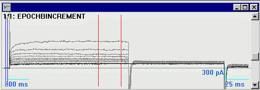
| step 11.2 | From the Conditioning menu choose family plot mode. |
| step 11.3 | In the 'input tool box' activate the 'Invert' and 'Zero' buttons, then drag 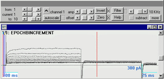
Eventually, use the 'amp' slide bar to amplify the records. |
| step 11.4 | Push the copy icon |
| step 11.5 | From the File menu choose new and in the dialogue box that pops up select 'drawing sheet'. |
| step 11.6 | Push the paste icon |
| step 11.7 | Double click on one of the calibration bars (axes) of the figure and fill-in the 'axes' dialogue box as shown below. By setting the Y-coordinate limits, we cut off the transients as it were.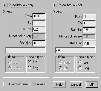 Then push 'OK'. Then push 'OK'.The graph on the drawing sheet will then look like: 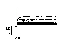 |
| 12 Creating an IV curve from impulse data. | |
| step 12.1 | Load the file step11.dat if it is not already loaded, activate the 'invert' and 'zero' buttons in the input tool box and move the blue ('zero' window) and red ('action' window) lines as shown below:
 |
| step 12.2 | From the Extract menu select create XY line plot. The 'Create Plot' dialogue window appears. Consult the paragraph 'Creating a graph directly from input data' to know the details. For now, select the options as shown below (do not forget to set the 'copy to clipboard' option):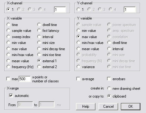 |
| step 12.3 | Activate the drawing window from the previous exercise by clicking on its title bar (or open the file). Then click left of the figure (that is where our IV curve will be pasted) and push the paste icon in the program icon bar. The result will be: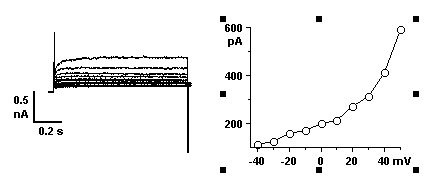 |
| step 12.4 | Now modify the axes by double-clicking on one of the two. Fill in the axes dialogue window as follows: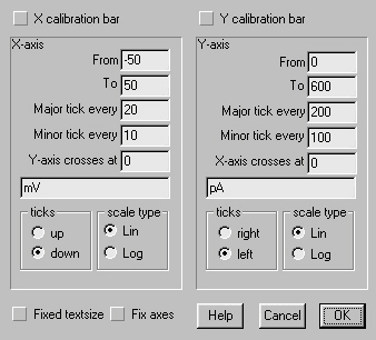 Then push 'OK'. Then push 'OK'.The graph on the drawing sheet will look like: 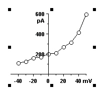 |
| 13 Leak subtraction. | |
| step 13.1 | Load the file step11.dat if it is not already loaded, activate the 'invert' and 'zero' buttons in the input tool box and move the blue ('zero' window) and red ('action' window) lines as shown in step 12.1. |
| step 13.2 | Choose Subtraction setup from the Conditioning menu. A dialogue window appears. Select the options as shown below: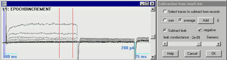 2 nS leak is now subtracted from each trace. Push the 'OK' button. Note that the 'subtract' option in the input window tool box is set. If it is not: set it. |
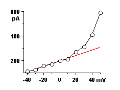
| step 13.3 | Proceed as in steps 12.2 through 12.4. The result will be: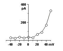
Note that the leak conductance could have been estimated by fitting (see step 4 on how to fit) the first 5 points in figure 10.4 by a straight line as shown below:
The tangent of the fitted red line is 2.214 nS. |
| 14 Creating an IV curve from ramp data. | |
| step 14.1 | Open file 'step14.dat'. This file should reside in your program directory. If you can't find it, you may download it here. This file contains one sweep, two input channels. Channel 1 contains the current response to a voltage ramp, while channel 2 shows the voltage ramp itself. For channel 1 choose the following settings: Then push the |
| step 14.2 | Move the red vertical lines (action window, or part of the trace that will be used for the analysis) for both input channels simultaneously. This is done by dragging the red lines while keeping the <CTRL> key on your keyboard depressed. Their positions should be like: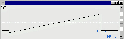 |
| step 14.3 | Although it is not needed for the analysis, the two input channels may be visualised simultaneously by selecting multi channel plot mode from the Conditioning menu: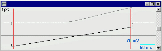 |
| step 14.4 | From the Extract menu select create XY line plot. The 'Create Plot' dialogue window appears. We'll plot the current of channel 1 as a function of the voltage of channel 2 as follows:  The 'max 200 x-points' has been set to limit the number of points in the graph A new drawing sheet is created with the following figure: 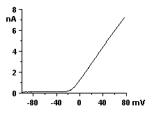 |
| 15 Channel analysis: the probability density histogram. | |
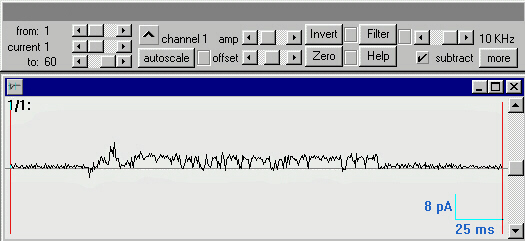
| step 15.1 | (Down-)load file 'step15.dat'. This file should reside in the program directory. It contains voltage-evoked channel openings. Choose the following settings in the input tool box and change amplification 'amp' as necessary: 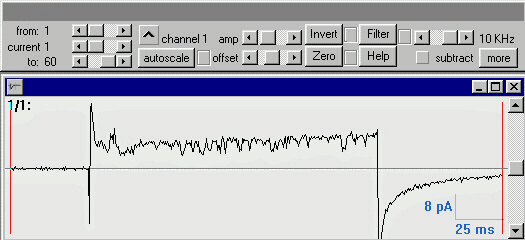 |
| step 15.2 | First we have to get rid of the stimulation transients. Choose subtraction set-up from the Conditioning menu. The 'subtraction' dialogue window appears: 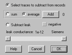
Move to record number 13 using the 'from' slidebar in the input tool box. Push the 'Add' button in the 'subtraction' dialogue window. Then move to record number 19 and again push the 'Add' button. Push the 'OK' button. |
| step 15.3 | Drag the red action window delimiters as shown below: 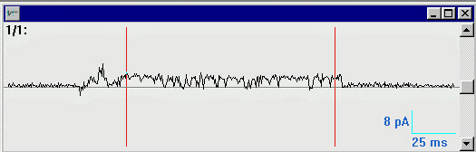 |
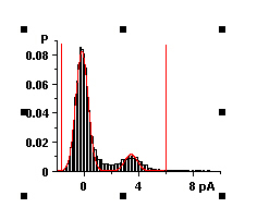
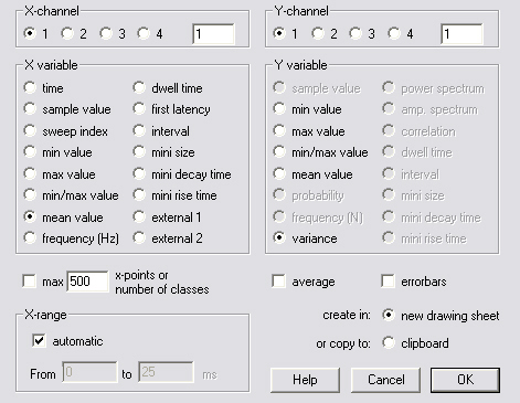
| step 15.4 | From the Extract menu select create XY line plot. The 'Create Plot' dialogue window appears. We'll create the current-density histogram as follows: 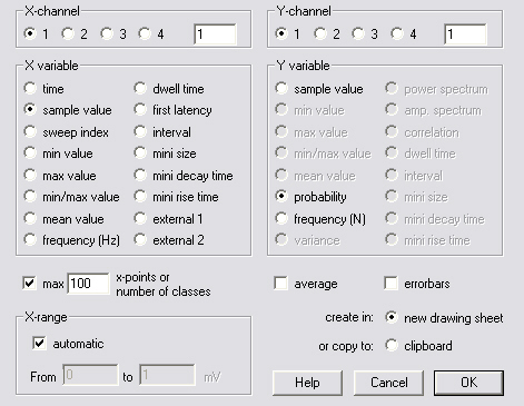 After having pushed the 'OK' button, a new drawing sheet is created with the probability histogram, that will be shown a few images further on. Now we'll fit the histogram with a dual Gaussian function. (See step 4 for a more detailed example of curve fitting).
 |
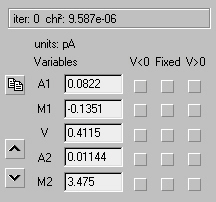
| step 15.5 | Double-click on the histogram. The 'Curve properties' dialogue window appears. Set the 'fit range' from -1.5 to 6 (pA) approximately. Then push the 'Function' button. The 'Fit' dialogue window pops up: 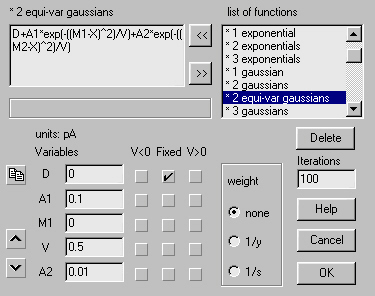 Select the '*2 equi-var gaussians' function (2 Gaussians with the same variance) and push the '<<' button. This is a rather non-linear function and during the fitting iterations the routine gets easily stuck at a local minimum. So we have to set the starting parameters close to the absolute minimum as shown in the above figure. The parameter 'D' is offset which needs to be fixed at '0' (we do not fit this parameter). 'A1' and 'A2' are the amplitudes of the two Gaussians. From the histogram we see that they are approximately P=0.1 and P=0.01. 'M1' is the mean of the first Gaussian, the closed channel state, and hence 0 pA. To be able to see the remaining parameter to fit, 'M2', push the 
|
| 16 Channel analysis: the dwell time histogram. | |
| step 16.1 | Load file 'step15.dat' and follow steps 15.1 and 15.2 (leak subtraction). |
| step 16.2 | From the Conditioning menu select Idealise channels. The 'idealise' dialogue window pops up: 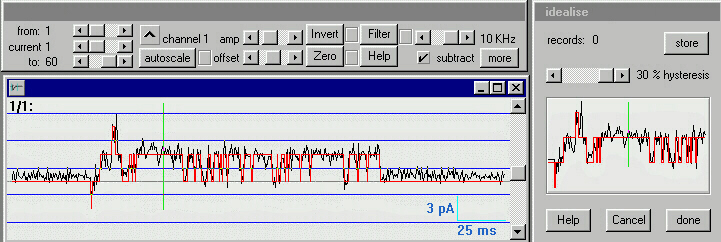 Drag one of the horizontal blue lines (thresholds) up or down until the above image is realised. One can estimate the required position of the thresholds by eye or use the information that we obtained in step 15. In step 15 the unitary current was estimated to be 3.6 pA. The size of the unitary current (as depicted by the red line) is shown in the program status bar (that is the bottom bar of the program window). Move the thresholds until it shows: Set The hysteresis level in the "idealise" dialogue box at its maximum (30%). Then push the "store" button. The Idealised trace is now stored in a temporary file and the next sweep is shown. Either push "store" again, or hit the <RETURN> key until the end of the file is reached. Then push "done". The "save file" dialogue window pops up. Save the idealised data under "step15.cha" (the default).Close the file "step15.dat", since we do not need it anymore. |
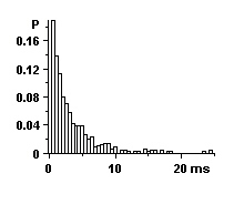
| step 16.3 |
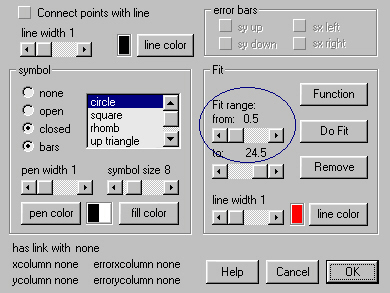
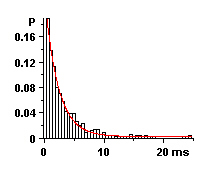
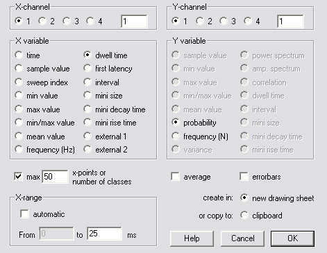 From the Extract menu select create XY line plot. The "Create Plot" dialogue window appears. We'll plot a dwell time histogram using the settings shown here on the left. Set the number of classes to 50 and the X-coordinate range to 25 ms, then push 'OK'. 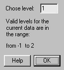
A new dialogue window appears: choose level number 1 (1 channel open) and push 'OK' |
| 17 Simulate channel activity. | |
| step 17.1 | From the File menu choose new. |
| step 17.2 | In the 'Select File Type' dialogue window, choose 'spreadsheet' and push 'OK'. A blank spreadsheet is created. |
| step 17.3 | Enter numbers in the spreadsheet cells as shown in the figure: 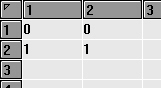 This spreadsheet contains the information to simulate a channel that has two states. The numbers on the diagonal indicate whether the states are open(1) or closed(0). Hence state 1 is closed and state 2 is open. The off-diagonal cells contain the rate constants (in 1/seconds) between the states. The rate constant from state 1 to state 2 is 1 and the reverse rate constant is 0. It is a very simple model. This spreadsheet contains the information to simulate a channel that has two states. The numbers on the diagonal indicate whether the states are open(1) or closed(0). Hence state 1 is closed and state 2 is open. The off-diagonal cells contain the rate constants (in 1/seconds) between the states. The rate constant from state 1 to state 2 is 1 and the reverse rate constant is 0. It is a very simple model. |
| step 17.4 | 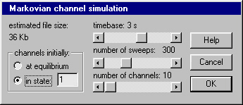 To start simulation, either select a single cell, no matter which, or select the four cells (no more and no less). Then choose Markov simulation>channels from the Math menu.First the 'save' dialogue window asks for a filename. Enter '10ch' as the new filename and push OK. Then fill in the nex dialogue window that pops up as shown to the right and push the OK button when done. To start simulation, either select a single cell, no matter which, or select the four cells (no more and no less). Then choose Markov simulation>channels from the Math menu.First the 'save' dialogue window asks for a filename. Enter '10ch' as the new filename and push OK. Then fill in the nex dialogue window that pops up as shown to the right and push the OK button when done. |
The new file '10ch.cha' is created. The result may resemble: 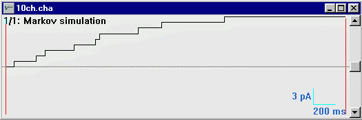 Hence at the beginning of the trace all chan-nels are closed, but when time proceeds, more and more open up. The program sets the unitary current arbi-trarily to 1pA. | |
| 18 Channel analysis: the variance to mean histogram. | |
| If the probability of channel opening varies within a trace (as in the case of a voltage-dependent channel that is subjected to a voltage jump), and if many such traces exist, then the number of channels and the single-channel conductance may be estimated by plotting the variance as a function of the mean current. In this example we'll use the 10ch.cha file that was created in the previous exercise. | |
| step 18.1 | Open the file 10ch.cha and place the red vertical lines (action window) at the extremes as in the figure in step 17.5. |
step 18.2 |
Select Create XY line plot from the Extract menu and set the entries in the dialogue window that pops up as shown to the right and push the OK button. |
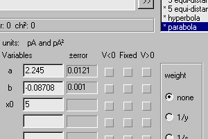
| step 18.3 | According to Neher, E. & Stevens, C. F. (1977) Conductance fluctuations and ionic pores in membranes. Annual Review of Biophysical Bioengineering 6, 345-381, the relation between variance (s(p)) and mean (m(p)) is:s(p) = i.m(p)-m2(p)/N, with p the probability of channel opening, i the unitary current and N the total number of channels. 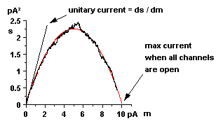 Differentiation of s with respect to m gives: ds/dm=i -2.m/N. Hence at zero mean current (p=0): ds/dm=i. Fitting the histogram with a parabola: s(x)=a+b.(x-x0)2 gives two equations: at x=0: ds/dx = -2.b.x0 = i and at the intersection of the parabola with the y=s(x)=0 axis: x=N.i. Therefore, fit the histogram with a parabola. The result should be similar to the figure to the left. Differentiation of s with respect to m gives: ds/dm=i -2.m/N. Hence at zero mean current (p=0): ds/dm=i. Fitting the histogram with a parabola: s(x)=a+b.(x-x0)2 gives two equations: at x=0: ds/dx = -2.b.x0 = i and at the intersection of the parabola with the y=s(x)=0 axis: x=N.i. Therefore, fit the histogram with a parabola. The result should be similar to the figure to the left.
Hence the unitary current is 2*0.087*5 = 0.87 pA and the total number of channels is estimated to be 10/0.87=11.5. We know from the previous exercise that these values should have been 1 pA and 10 channels respectively. |
| 19 Measuring the cell capacitance. | |
| There are several ways to measure cell capacitance. The method followed in this exercise is rather simple and assumes that leak is not very large and series resistance negligible. Capacitance C (in Farad) is related to charge Q (in Coulomb) and voltage V (in Volt) by C=Q/V. Hence, when in voltage-clamp, it suffices to measure the integral of the current in response to a known voltage jump to obtain the cell capacitance. | |
| step 19.1 | Load the file 'step19.dat' which should reside in your Electrophy directory or download it here. The file contains only one trace. It shows a capacitive current that was obtained with a voltage jump from -90 to -80 mV. Check the zero button and position the blue vertical lines (the 'zero' window) as shown. The average value between the blue lines is subtracted from the entire trace, making sure that at the end of the pulse the current is 0. 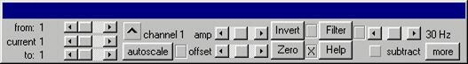 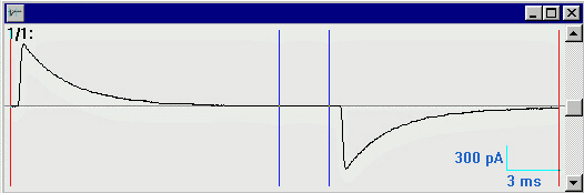 |
| step 19.2 | Now we'll integrate the current trace numerically. Push the 'more' button in the input tool window. The alternate input tool window now shows. 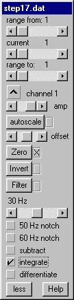
Check the 'integrate' checkbox and increase amplification using the 'amp' slide bar. Note that the Y-axis is now calibrated in pC (pico-Coulomb). |
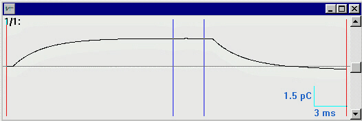
| step 19.3 | In order to know the total charge accumulated by the cell membrane capacitance click anywhere near the plateau phase of the integral. A cursor appears: 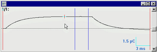 and the status bar (the lower bar in the program's window) reads: Hence the total charge is 1.99 pC at 10 mV, which gives C=1.99e-12/10e-3 F = 199 pF. Very often the picture is a little less perfect as in this example and just a bit of leak current could cause the integral trace just before the onset of the voltage jump to deviate from 0. In that case we need to take the difference of the integral just before the pulse and the integral at the plateau phase. To do so: |
| step 19.4 | Click at the beginning of the trace, release the mouse button and move the second cursor that appears to the plateau phase as in the figure below: the status bar now reads: It shows the X and Y coordinates of the two cursors and their difference i.e. 1.98 pC The positions of the cursors in the input window may be transferred to a spread sheet (which can be useful if the capacitances of many cells need to be determined) by pressing the 'T' key on the keyboard or the right mouse button:  |
Thanks are due to those who have stimulated the development of this program with their useful comments.
I'd like to thank in particular Joseph Skopp at the University of Nebraska who sent me his error function routine.
This program contains the sixth public release of the Independent JPEG Group's free JPEG software. This software is the work of Tom Lane, Philip Gladstone, Luis Ortiz, Jim Boucher, Lee Crocker, Julian Minguillon, George Phillips, Davide Rossi, Ge' Weijers, and other members of the Independent JPEG Group.IJG is not affiliated with the official ISO JPEG standards committee.