The spreadsheet
 A spreadsheet is a text document that organises data in columns and rows. A blank spreadsheet can be created by using the File>new menu option. An existing spreadsheet is read by using the File>open option from the menu or clicking the open file icon. From the open file dialogue window select type=Spreadsheet files. Tab-delimited or comma-delimited files need to have the extension *.txt or *.etf (extended text file) in order to be read. Because software that comes with some laboratory equipment saves data in MS-Excel *.xls format, Electrophy reads this file format, although without parsing most of the spreadsheet functions that it may contain. It just reads the numerical result.
There are two ways to enter data in a spreadsheet cell. i) Click on the cell you wish to edit and type the new text. Upon pressing the return key or one of the arrows on the keyboard the old text is replaced by the new text. Depending on which key was pressed, a next neighbour cell is highlighted. ii) Click on the cell you wish to edit and then click in the edit box
Numerical data may be entered in one of three formats: 1) in floating point format (e.g. 1.23e-5). 2) in "time" format hh:mm:ss, where hh=hours, mm=minutes and ss=seconds. hh,mm and ss may be floating point. The latter is useful only to enter fractions of a second (e.g. 0:0:0.66). The "time" format may not be used in formulas. Hence "12:30:00" is OK, but "=12:30:00" is not. instead, use the time() function to enter time data in formulas. 3) a date may be entered as "dd/mm/yyyy", where dd=days is an integer value between 1 and 31, mm=month is an integer value between 1 and 12 and yyyy is the year. The "date" format may not be used in formulas. Hence "24/02/1999" is OK, but "=24/02/1999" is not. Instead, use the date() function to enter date data in formulas

Selecting multiple cells.
There are two ways to select multiple cells.
i) Click on a cell and, while maintaining the left mouse button depressed, move the mouse pointer.
ii) Click on a cell and release the left mouse button. Then press the shift key and click on a second cell, release the left mouse button and release the shift key. Now multiple cells are highlighted.
Selecting rows.
Click on a row key (showing the row index). To select multiple rows, click in a row key and move the mouse while keeping the left mouse button depressed. A second way to select multiple rows is to click on a row key and then on a second key, while depressing the shift key on your keyboard.
Selecting columns.
Click on a column key (showing the column index). To select multiple columns, click in a column key and move the mouse while keeping the left mouse button depressed. A second way to select multiple columns is to click on a column key and then on a second key, while depressing the shift key on your keyboard. The third way is to click on a column key and then to click on other column keys while keeping the <Ctrl> key depressed. This option is available only for multiple column selection and results in a selection of columns that is not contingent.
Formulas
Create equations by typing the "=" character as the first character in a spreadsheet cell.
The following math functions are supported
Several functions such as SUM() and SEM() require a range of spreadsheet cells as argument. There are two ways to enter such a range in a formula: i) Type it (e.g. "mean(C2:L2,C2:L300)"), N.B.: do not type the quotation characters, or ii) in the spreadsheet edit box
Parameters
Many functions, like sin(), only demand a single parameter. If you wish this parameter to be a reference rather than a number, type for instance "=sin[C2:L3]". A second way to enter the reference is the following: in the edit box![]() type "=sin" (a bracket is not necessary here), then right-button click the cell that contains the argument. The text string will then read: "=sin[Cn:Lm]", where n and m are the indices of the cell containing the argument. Observe that the type of bracket used is not important for the mathematical result: "{", "(" and "[" are OK. However for mouse-editing they make a difference: only the reference to a single cell is entered after a square bracket "[" or any symbol other than "{" or "(", whereas a range of cells will appear after "{" or "(".
type "=sin" (a bracket is not necessary here), then right-button click the cell that contains the argument. The text string will then read: "=sin[Cn:Lm]", where n and m are the indices of the cell containing the argument. Observe that the type of bracket used is not important for the mathematical result: "{", "(" and "[" are OK. However for mouse-editing they make a difference: only the reference to a single cell is entered after a square bracket "[" or any symbol other than "{" or "(", whereas a range of cells will appear after "{" or "(".
Conditional variants
All functions that take a range of cells as an argument have a conditional variant that takes a range, a condition (e.g. >24) and a cell as arguments. For example: "sum((C2:L2;C2:L300);>24;[C20:L2])". The cell [C20:L2] is the top left cell of a second range of cells that has the same dimensions as the first one. Thus, to each cell in the first range corresponds a cell in the second range. If the content of the cell in the second range satisfies the condition, then the content of the cell in the first range contributes to the sum. In the example at hand, the content of the cell in the second range of cells has to be superior to 24 if the cell in the first range is to contribute to the function. The condition consists of one of the operators =, >, <, >= or >= followed by a (floating point) number.
How to modify the range of cells in a function.
Again there are two ways to do this:
i) re-type the new range, or
ii) Click on the cell containing the function. In the edit box![]() , place the cursor anywhere between the brackets delimiting the function's argument. Then right-button-click the new first cell in the spreadsheet and move the mouse while maintaining the right button depressed. The new range replaces the old one automatically.
The reference of single-argument functions can be changed similarly.
, place the cursor anywhere between the brackets delimiting the function's argument. Then right-button-click the new first cell in the spreadsheet and move the mouse while maintaining the right button depressed. The new range replaces the old one automatically.
The reference of single-argument functions can be changed similarly.
What happens if you copy and paste a formula?
If you paste a formula onto a cell in the same or another spreadsheet, the column and line (row) indices are incremented or decremented such that the relative distance between the cell that receives the formula and the cell(s) the formula is referring to remain(s) the same in the original and the copy. An example explains this more clearly. Say a cell at column 2, line 3 contains the function "=SIGN[C1:L5]". After having copied the cell you paste it at column 2, line 4. The function in the receiving cell will then read: "=SIGN[C1:L6]". If you don't want the index to change when pasting, put a "$" sign in front of the index in the original cell (e.g. "=SIGN[C1:L$5]").
What will happen to references if you delete or insert spreadsheet cells?
If a (number of) cell(s) is deleted or inserted, the cells below or to the right of the deleted/inserted cell(s) will shift position. The references contained in the shifted cells are updated such that they still refer to the same cell as before, with one exception: cells referring to deleted cells will not be updated. Hence, the former cells will refer to cells that have taken the position of the deleted cells. Electrophy does not warn you of such a mishap, unless the formula containing the reference has become nonsense (not because it can not detect such events, but to prevent too much mouseclicking).
How to create a function that depends on a running index.
Either the current column index or the current line index can be used as a running index to create "functions". To do this use "cin" (column index) or "lin" (line index) in your function e.g. "=sqrt[3+lin*3] will result in "3" if the cell containing the function is at line 2. It will return "6" if it is at line 11.
What is the function "cell()" good for?
Cell(c;l) retrieves the contents of a cell at column c and line (row) l. As c and l may be functions themselves, the indices may thus be the result of a calculation or a Boolean expression.
References in the functions cell(c;l), getlnum(c;n;r0), getcnum(l;n;c0), getltext(c;x;r0) et getctext(l;x;c0) The values of c and l in those functions that take a column or line index as argument could present a problem if one adds or removes cells from the spreadsheet. For example, if the cell [C3:L3] contains "=cell(10;10)" and the cell [C10:L10] contains the value 12, The result shown in cell [C3:L3] will be 12. Now if we add a new column in between columns 3 and 10, then the cell containing the value 12 will not be at [C10:L10] but at [C11:L10]. Therefore, cell(10;10) will return in general an other number than 12. Furthermore, if one copies cell [C3:L3] onto cell [C5:L3], the result shown in the two cells will be identical as both contain "=cell(10;10)". Often one wishes that the references to columns and lines in the functions cell(), gecnum() etc behave similar to the ranges and cells described a few paragraphs above, i.e. they adapt their indices if one adds or removes spreadsheet cells. To indicate an adaptable index in those functions, use the prefixes C and L. Hence, to indicate that the arguments in the function "=cell(10;10)" have to be adaptable, use the notation: "=cell(C10;L10)". In the latter case, "=cell(C10;L10)" becomes identical to [C10:L10].
Self-referencing
Self referencing as for example in "=1+cell(cin;lin)", is not recommended and in general will be punished by unpredictable results. However, no error message is issued, since it is possible to construct perfectly stable systems of cells that contain self references or circular references.
Date format
The program internally stores dateThe date format is of the form "dd/mm/yyyy" where dd is days (1-31), mm the month of the year (1-12) and yyyy the year according to the Gregorian calendar. Example: 12/10/2016. data as the number of days since 31st Dec of the year 0 according to the Gregorian calendar. This number of days may be retrieved using the function "float()". In general, math operations on dates give results that are not meaningful. There are a few exceptions. Suppose two spreadsheet cells, [C1:L1] and [C2:L1], each contain a date, then "=float([C1:L1]-[C2:L1])" returns the difference in days between the two dates. With the functions year(n) and month(n) one can add (or subtract) a certain number of years or months to (from) dates. Hence, if cell [C1:L1] contains a date, say 12/10/1999, then the expression "=[C1:L1]+year(2)" will return 12/10/2001. The addition of dates, years, months and days is neither commutative nor associative. As the program's formula parser supposes the normal associativity and commutativity rules, the user should explicitly indicate the order in which math operations have to occur. For example "=[C1:L1]+year(2)" will not give the same result as "=year(2)+[C1:L1]". Typing "=[C1:L1]+year(2)+month(1)" is dubious since the parser may first add year(2) and month(1), applying the normal associativity rule for addition, before adding it to the date. To be sure of the result type "=([C1:L1]+year(2))+month(1)".
Slide bar
A horizontal slidebar ![]() is displayed in a spreadsheet cell when using the function "=SBAR(minimum,current value,maximum)". Minimum and maximum set the range of values the current value (or cursor position) may adopt. The initial "current value" is immaterial, but may not be left blank. The sbar() function may be part of a more intricate formula, e.g. "=1+sbar(0,5,10)", but it should appear only once in a spreadsheet cell. The resolution of the slidebar is 1/100, therefore clicking on one of the two gadgets
is displayed in a spreadsheet cell when using the function "=SBAR(minimum,current value,maximum)". Minimum and maximum set the range of values the current value (or cursor position) may adopt. The initial "current value" is immaterial, but may not be left blank. The sbar() function may be part of a more intricate formula, e.g. "=1+sbar(0,5,10)", but it should appear only once in a spreadsheet cell. The resolution of the slidebar is 1/100, therefore clicking on one of the two gadgets ![]() at the extremities of the slide bar will increment or decrement the current value by 1% of the difference between maximum and minimum. Clicking between an endpoint gadget and the central cursor will change the current value by 10%. The central cursor may be moved by dragging it with the mouse. As with all other spreadsheet functions, the sbar() arguments may be functions or references. However, it is useless to assign a function or reference to "current value" as it will be replaced by a floating point number as soon as the user actions the slidebar.
The output of a spreadsheet cell containing a slidebar may be used for example as a parameter in a function defining a column of spreadsheet cells. If this column is linked to a graph on a drawing sheet, then moving the slidebar cursor will change the data in the spreadsheet and hence the graph. See the "doc" file in the program directory for an example.
at the extremities of the slide bar will increment or decrement the current value by 1% of the difference between maximum and minimum. Clicking between an endpoint gadget and the central cursor will change the current value by 10%. The central cursor may be moved by dragging it with the mouse. As with all other spreadsheet functions, the sbar() arguments may be functions or references. However, it is useless to assign a function or reference to "current value" as it will be replaced by a floating point number as soon as the user actions the slidebar.
The output of a spreadsheet cell containing a slidebar may be used for example as a parameter in a function defining a column of spreadsheet cells. If this column is linked to a graph on a drawing sheet, then moving the slidebar cursor will change the data in the spreadsheet and hence the graph. See the "doc" file in the program directory for an example.
The Edit menu
The Edit menu allows you to copy, paste, delete and otherwise manipulate data in the spreadsheet. As the functions of most of the menu items are self evident, they will not be described here. Even so, a few points merit attention:
* When pasting the clipboard contents on the spreadsheet, it suffices to click the top left cell where you wish to paste. The structure of the clipboard contents will determine how many cells will be modified.
* When pasting on the spreadsheet after having highlighted entire rows or columns, the paste becomes an "insert/paste". This is not a bug, but a shortcut.
* Copy vs. Copy values. When copying text from a spreadsheet cell you copy the text that has been previously entered in the cell. This text might have been a formula (e.g. "=exp(-20*[C1:L1])"). When pasting the contents of the clipboard, the new cell will contain "=exp(-20*[Cn:Lm])", where n and m will depend on source and destination. If you wish to copy (and thus paste afterwards) the numerical result of the equation rather than the equation itself, use copy values. Note that this is a different approach than used by Microsoft Excel, where you make this choice upon pasting rather than upon copying. * Copy L <--> C (or <Ctrl> Q) copies the selection, interchanging columns and rows.
* Delete removes cells from the spreadsheet, while Clear replaces them by empty cells.
* When deleting, be aware that references to the deleted cells may not be valid anymore. Electrophy does not protest, unless formulas really make no sense.
Delete empty cells
The Delete empty cells command removes all empty cells from the selected column(s), shifting cells below the deleted cell upwards.
Replace
When using the Replace menu item, formulas will be affected too. Hence "Replace 4 by 7" will change references if they contain the number 4.
Select all (or ^A) selects the whole spreadsheet
Finder (or ^F)
Finds text on your sheet. The following dialogue box comes up after selecting this menu item:

Type the text to find in the edit box![]() , select either "Search selection" to search the highlighted selectoin or the entire spreadsheet. Choose to search in either forward or backward direction. If the box
, select either "Search selection" to search the highlighted selectoin or the entire spreadsheet. Choose to search in either forward or backward direction. If the box![]() "Respect case" is not checked, upper or lower case will not matter. The finder will search for an exact match if "Strict" is checked, i.e. searching for "fun" will not find "fundamental" in that case.
"Respect case" is not checked, upper or lower case will not matter. The finder will search for an exact match if "Strict" is checked, i.e. searching for "fun" will not find "fundamental" in that case.
Remove links
The Remove links item will remove all links of the selected columns with all graphs in all drawing sheets. To remove the link with only one graph, select the graph and then choose the Edit>Remove Link item from the drawing sheet menu. More on links elsewhere.
Edit mode without copy
Spreadsheet editing may become somewhat slow if the spreadsheet contains much data. Speed may increase considerably if the undo backup buffer need not to be maintained up to date. Check the Edit mode without copy option to achieve this. The price to pay is that Undo will then not always be available.
Comma-delimited file
If a Comma-delimited text file was read onto the spreadsheet, then the Comma-delimited file menu item will be checked. Uncheck this option if you wish to save the file in TAB-delimited format later. Note that if you save a file in Comma-delimited format, that commas which may occur in spreadsheet cells will be treated as column separators the next time you reload the file.
Change font size
The font size of the spreadsheet may be changed using the Change font size option from the Edit menu. After selection of this option a small dialogue box comes up in which the new size can be set. Note that the width and the height of all cells on the spreadsheet will be set to the new default sizes corresponding to the chosen font dimensions.
Save Prefs
The Save Prefs menu item writes the current preferences to disk.
These preferences are:
The current window dimensions,
The default column width and line height,
The text font,
The current page format, e.g. A4, US letter etc,
The current page orientation, i.e. portrait or landscape,
The default number of decimals displayed,
The editmode with/without copy.
Newly created windows will have these parameters per default.
The Fill menu
In order to copy the contents of a single cell to a range of cells use the Fill>right or the Fill>down commands. First, left-mouse-button select a range of cells and then issue one of the commands from the Fill menu.
Right copy will copy the contents of the left-most cells to the right.
Right value will copy the numerical value (rather than the formula, if be) to the right.
Right increment will copy the numerical value of the left-most cell to the right, incrementing by 1 as it proceeds to the right.
Right decrement does similarly, but decrementing by 1.
Right interpolation fills empty cells (and only empty cells) by interpolating between the numerical values of non-empty cells that need to be contained in the highlighted selection. If the beginning and/or end of the range of selected cells is empty, extrapolation is carried out if possible. Extrapolation is carried out only if the highlighted selection of cells contains at least two non-empty cells. Cells containing non-numerical text are considered to represent the value 0 (zero).
If you wish to carry out the same fill command with a next selection of cells, right-mouse-button select the new range and the last issued fill command will be carried out automatically.
Note that right-mouse select applies to the fill menu only. Hence, it does not repeat for instance a previous Edit>delete action. Use the repeat icon![]() in the icon bar or Edit>Repeat last from the menu to repeat edit actions.
The Fill>down commands behave analogously by copying the contents of the top-most cell(s) downward.
in the icon bar or Edit>Repeat last from the menu to repeat edit actions.
The Fill>down commands behave analogously by copying the contents of the top-most cell(s) downward.
Demo:
"Create a linked plot" is better viewed full screen
The Modify/Stats menu
Line plot, Bar plot and Wind rose plot
These menu items are used to create a graph on a drawing sheet. Before issuing one of these two commands you need to indicate which of the columns contain the data to be plotted. There are two ways to do this:
Method 1) select a column that contains data for the x-axis by clicking on the column key at the top of the spreadsheet and then select Modify/Stats>Set X-column from the menu. This menu item may also be used to select the column containing the angular coordinates (in radians) for a wind rose plot. Then select a column that contains the y-data and choose Modify/Stats>Set Y-column from the menu. Select Modify/Stats>Set Z-column from the menu if you'd like to create an XYZ plot. Optionally, you may select a column that contains values for the error bars (a symbol whose size indicates the statistical error in the associated y-data point) by choosing the Modify/Stats>Set Error-column from the menu. Hence, this method allows you to select at maximum four columns and the order of the columns is unimportant.
Method 2) select a number of columns that you wish to use for your graph. Then, when you issue the Plot command a dialogue window will pop up asking you to specify which of them contain x, y, z or error data. Here the order of columns is important.
An x-column (there may be more than one) has to precede the associated y- and z-column(s). A z-column should be in between an x and one or more y-columns. An error column refers to the column preceding it. Hence, if column 1 contains x-data and column 2 error data, the error bars will be plotted horizontally as they are assumed to refer to errors in the x-data. Two x-columns have to be separated by at least 1 column containing y-data.
Use the left ![]() and right button
and right button ![]() in the dialogue box to go to the next or previous column.
Create histogram in a
in the dialogue box to go to the next or previous column.
Create histogram in a ![]() new document or on the
new document or on the ![]() clipboard. By default, the histogram will be created in a drawing window of its own.
3D plots are created by selecting at least three columns, the first containing the x coordinates, the second the z coordinates and the third the y coordinates. An x-column may be followed by more z-columns. A z column may be followed by more y-columns. The 3D plot can be rotated once it has been created by first selecting the 3D plot and then the rotation tool
clipboard. By default, the histogram will be created in a drawing window of its own.
3D plots are created by selecting at least three columns, the first containing the x coordinates, the second the z coordinates and the third the y coordinates. An x-column may be followed by more z-columns. A z column may be followed by more y-columns. The 3D plot can be rotated once it has been created by first selecting the 3D plot and then the rotation tool ![]() . A horizontal movement turns the graph around the vertical axis. A vertical movement turns the graph around the horizontal axis. Horizontal movements are ignored if the shift key is depressed. The graph turns around the axis perpendicular to the screen if the <Ctrl> key is depressed. Rotations can also be carried out using the Tools>Rotate menu item.
To transport the new histogram to another drawing sheet, select the histogram by clicking once on it, then copy or delete it (<Ctrl> C or <Ctrl> X or the Copy or Delete command from the Edit menu) and paste it (<Ctrl> V or the paste command from the Edit menu) onto the other drawing sheet.
If you select the "create histogram on clipboard" option, the histogram will be created on the clipboard. This is, however, less intuitive as nothing seems to happen until you issue the paste command after having selected a drawing sheet.
. A horizontal movement turns the graph around the vertical axis. A vertical movement turns the graph around the horizontal axis. Horizontal movements are ignored if the shift key is depressed. The graph turns around the axis perpendicular to the screen if the <Ctrl> key is depressed. Rotations can also be carried out using the Tools>Rotate menu item.
To transport the new histogram to another drawing sheet, select the histogram by clicking once on it, then copy or delete it (<Ctrl> C or <Ctrl> X or the Copy or Delete command from the Edit menu) and paste it (<Ctrl> V or the paste command from the Edit menu) onto the other drawing sheet.
If you select the "create histogram on clipboard" option, the histogram will be created on the clipboard. This is, however, less intuitive as nothing seems to happen until you issue the paste command after having selected a drawing sheet.
After being drawn, the graph will be linked to the columns in the spreadsheet, meaning that a modification in one of the columns will alter the graph ![]() . Columns that maintain a link with a graph are marked by a '°' character in front of the column index. The link can be removed by either clicking on the graph and selecting Edit>Remove Link from the drawing sheet menu or by selecting the columns and selecting Edit>Remove Links from the spreadsheet menu. The latter action will also remove links with other graphs on other drawing sheets if they exist. More on links elsewhere.
. Columns that maintain a link with a graph are marked by a '°' character in front of the column index. The link can be removed by either clicking on the graph and selecting Edit>Remove Link from the drawing sheet menu or by selecting the columns and selecting Edit>Remove Links from the spreadsheet menu. The latter action will also remove links with other graphs on other drawing sheets if they exist. More on links elsewhere.
Creating graphs with the X-axis labels in timeThe time format is of the form "hh:mm:ss" where hh is the number of hours, mm minutes and ss the number of seconds. example: 10:32:59 or dateThe date format is of the form "dd/mm/yyyy" where dd is days (1-31), mm the month of the year (1-12) and yyyy the year according to the Gregorian calendar. Example: 12/10/2016. format.
If a new graph is created from spreadsheet columns, where the column furnishing the X data is entirely in timeThe time format is of the form "hh:mm:ss" where hh is the number of hours, mm minutes and ss the number of seconds. example: 10:32:59 or dateThe date format is of the form "dd/mm/yyyy" where dd is days (1-31), mm the month of the year (1-12) and yyyy the year according to the Gregorian calendar. Example: 12/10/2016. format, then the X-axis labels will be in timeThe time format is of the form "hh:mm:ss" where hh is the number of hours, mm minutes and ss the number of seconds. example: 10:32:59 or dateThe date format is of the form "dd/mm/yyyy" where dd is days (1-31), mm the month of the year (1-12) and yyyy the year according to the Gregorian calendar. Example: 12/10/2016. format too. Double clicking on one of the axes in the graph will activate the Axes dialogue box as usual. Note however that the x-coordinates are now in timeThe time format is of the form "hh:mm:ss" where hh is the number of hours, mm minutes and ss the number of seconds. example: 10:32:59 or dateThe date format is of the form "dd/mm/yyyy" where dd is days (1-31), mm the month of the year (1-12) and yyyy the year according to the Gregorian calendar. Example: 12/10/2016. format. If the user enters a floating point number (rather than a time or a date) in one of the X-axis edit box![]() es, then a new dialogue box will pop up upon exit of the Axes dialogue box. In this box the user indicates if the graph should remain in timeThe time format is of the form "hh:mm:ss" where hh is the number of hours, mm minutes and ss the number of seconds. example: 10:32:59/dateThe date format is of the form "dd/mm/yyyy" where dd is days (1-31), mm the month of the year (1-12) and yyyy the year according to the Gregorian calendar. Example: 12/10/2016. format or should be converted to floating point (seconds/days). To convert the X-axis from floating point (seconds/days) to timeThe time format is of the form "hh:mm:ss" where hh is the number of hours, mm minutes and ss the number of seconds. example: 10:32:59/dateThe date format is of the form "dd/mm/yyyy" where dd is days (1-31), mm the month of the year (1-12) and yyyy the year according to the Gregorian calendar. Example: 12/10/2016. format do similarly (hence type at least one entry in timeThe time format is of the form "hh:mm:ss" where hh is the number of hours, mm minutes and ss the number of seconds. example: 10:32:59 or dateThe date format is of the form "dd/mm/yyyy" where dd is days (1-31), mm the month of the year (1-12) and yyyy the year according to the Gregorian calendar. Example: 12/10/2016. format).
If the graph's X-axis is in dateThe date format is of the form "dd/mm/yyyy" where dd is days (1-31), mm the month of the year (1-12) and yyyy the year according to the Gregorian calendar. Example: 12/10/2016. format, the Axes dialogue box is slightly different from the usual one in that the major and minor tick size should be entered in multiples of years (y), months (m) or days (d). Since the length of years and months is not constant (leap years, February is shorter than December) this results in non-equidistant ticks in the graph.
es, then a new dialogue box will pop up upon exit of the Axes dialogue box. In this box the user indicates if the graph should remain in timeThe time format is of the form "hh:mm:ss" where hh is the number of hours, mm minutes and ss the number of seconds. example: 10:32:59/dateThe date format is of the form "dd/mm/yyyy" where dd is days (1-31), mm the month of the year (1-12) and yyyy the year according to the Gregorian calendar. Example: 12/10/2016. format or should be converted to floating point (seconds/days). To convert the X-axis from floating point (seconds/days) to timeThe time format is of the form "hh:mm:ss" where hh is the number of hours, mm minutes and ss the number of seconds. example: 10:32:59/dateThe date format is of the form "dd/mm/yyyy" where dd is days (1-31), mm the month of the year (1-12) and yyyy the year according to the Gregorian calendar. Example: 12/10/2016. format do similarly (hence type at least one entry in timeThe time format is of the form "hh:mm:ss" where hh is the number of hours, mm minutes and ss the number of seconds. example: 10:32:59 or dateThe date format is of the form "dd/mm/yyyy" where dd is days (1-31), mm the month of the year (1-12) and yyyy the year according to the Gregorian calendar. Example: 12/10/2016. format).
If the graph's X-axis is in dateThe date format is of the form "dd/mm/yyyy" where dd is days (1-31), mm the month of the year (1-12) and yyyy the year according to the Gregorian calendar. Example: 12/10/2016. format, the Axes dialogue box is slightly different from the usual one in that the major and minor tick size should be entered in multiples of years (y), months (m) or days (d). Since the length of years and months is not constant (leap years, February is shorter than December) this results in non-equidistant ticks in the graph.
Build wind rose plot


The number of classes represents the number of (red) spokes in the final figure to the right. A multiple of 4 is advised for aesthetic reasons. When combining data into classes, these data may be weighed by either the number of entries in the spreadsheet column (no weight, i.e. each entry has the same weight) or by the vector size of the entry.
Frequency histogram
Creates a frequency histogram or a probability-density histogram of the currently selected column. Only one column can be selected for this option. In the dialogue window that pops up, the minimum value and the maximum value in the column are indicated along with a suggested number of classes (bins) for the histogram. This number of classes is estimated using the equation: Nclass=1 + 3.322 10log(N), where N is the number of data points in the spreadsheet column. Check the "normalise" box if you wish to create a probability-density function, leave it unchecked otherwise.
Create polygon
To create a polygon for use on a drawing sheet, select two columns of data, the first containing the x-coordinates (in screen pixels) and the second containing the corresponding y-coordinates. Alternatively, the x and y columns may be selected using the Set X column and Set Y column commands from the The Modify/Stats menu. Then choose Create polygon.
Example:
| x column: | y column: | gives as result: | |
| =10*cos(0.5*pi) | =10*sin(0.5*pi) | ||
| =10*cos(1.3*pi) | =10*sin(1.3*pi) | ||
| =10*cos(0.1*pi) | =10*sin(0.1*pi) | ||
| =10*cos(0.9*pi) | =10*sin(0.9*pi) | ||
| =10*cos(1.7*pi) | =10*sin(1.7*pi) | ||
| =10*cos(0.5*pi) | =10*sin(0.5*pi) |
A few other examples are included in the file: "polygons.txt" in the program directory.
Note that the x & y coordinates (in screen pixels) of polygon on a drawing sheet may be copied to a spreadsheet using the copy
Curve comparison
There are many ways to check for statistically significant differences between curves. The one that is at the base of this menu option is relatively easy to understand, but it has its limits as well. Suppose that we have two or more sets of data that are all dependent on the same variable, X. Suppose further that the variations around the means of each f(X) are Gaussian and have statistical moments that are independent of X, that means amongst others that the standard deviation has to be the same for all f(X). Under these conditions we can test the hypothesis that, after subtraction of the means for each X, the residues of all curves belong to the same population with mean zero (see the figure below).

To implement this method, you have to furnish the original data in a particular format on a spreadsheet:.

The data should be orginised into columns. The first one (optional) gives the values on the abscissa (X), the following columns give the data corresponding to the first curve. In the figure, columns 3 through 6 define the curve corresponding to "condition A", columns 7 through 10 define the curve "condition B". Empty cells are allowed. Then select the columns making up the new graph:

Then isue the Curve comparison command from the Modify/Stats menu. A dialogue box comes up. Check "X" for the first column (which is in this example column 2), then click the ![]() arrow until you reach column 7 and push the
arrow until you reach column 7 and push the ![]() arrow. Note that columns 7-10 are now labelled "Y2". Check "Bar plot" and push "OK".
arrow. Note that columns 7-10 are now labelled "Y2". Check "Bar plot" and push "OK".

A new drawing sheet with a the graph is created as well as two columns of residues in the spreadsheet corresponding to Y1 ("condition A") and Y2 (condition B"). The statistical differences between the two columns are returned by the Get column stats routine (see the next entry).

Get Column Stats
After having selected one or two columns, this menu item pops up a box showing statistics of the column(s) including mean, estimation of the standard deviation, error of the mean and, in case of two columns, the Student's t-test probabilities with results for paired and unpaired tests. If the number of columns selected is larger than 2, the result of Fisher's F-test is returned (1 way anova). If the F-test gives a probability below 5%, then Tukey's multiple comparison test (q-test) is carried out as well. Paste the data on a spreadsheet (after having closed the dialogue box) to get all the statistics.
Student's Test

If only population means, Standard deviations (SDs) and number of samples of two populations are known, and not the data themselves, then this menu item can calculate the t-value and the probability (P) that the two populations are identical. If the "population 2" box is unchecked, then the probability that the mean of population 1 is identical to 0 is calculated.
When you push the "done" button, the result is copied to the clipboard, such that it may be pasted on a document (e.g. spreadsheet).
Chi-2 Test

Select a rectangular range of spreadsheet cells that contain your data and issue the Chi-2 Test command. The rectangle has to be at least 2x2 cells otherwise you will get the "Degrees of freedom equals 0" message. For instance if you wish to test the hypothesis that hair colour is independent of sex and you have found the following population samples:
Males: black hair 32, brown hair 43, blond hair 16 and
Females: black hair 55, brown hair 65, blond hair 64. Then select the range of spreadsheet cells as in the figure.
Hence, the hypothesis that sex and hair colour are independent should be rejected as its probability to be true is only P=0.01149.
Convert to polar notation
Converts two columns containing the x and y coordinates of two-dimensional vectors into polar notation (angle, vector length).
Convert to vector notation
Converts two columns containing two-dimensional vectors in polar notation (angle, vector length) into the x and y coordinates of these vectors.
Resize column/line length
Graphs that contain a lot of data points (>5000) slow down the process of data manipulation and in general are rather useless. If a link between the graph and columns in the spreadsheet exist, the number of data points can be reduced by choosing Modify/Stats>Resize column/line length from the menu. The number of data points will be reduced either by removing every n-th data point or by averaging n points. You can select the final number of points in the selection of spreadsheet cells (and hence the graph) by indicating it in the dialogue window that pops up.
Sort
Numbers in a range of selected spreadsheet cells can be sorted in ascending or descending order using this menu item. A dialogue window will ask you to give these details. If spreadsheet cells in more than one column are selected, the cells in the "key column" will be sorted and the data in the neighbouring cells in the same row (line) will be moved upwards or downwards along with the data in the "key column". Check the "1<a" box if you wish to change the order of numbers with respect to letters and words in the column. Per default numbers come after letters when sorting conventionally (first a then z). UP↑
Set Column integer Base
Per default, numbers are shown on the spreadsheet in decimal floating point format. To change this into an integer format with a different base select this menu item. In the dialogue box that comes up a choice between base 2 (digital), 8 (octal), 10 (decimal, floating point) and 16 (hexadecimal) can be made. The program\'s internal representation remains in decimal floating point, only the presentation in the column in question changes. It is thus easy to convert numbers of one base into another e.g. by copying a number in an octal column to a column in another format. Note that the column header shows "b2", "b16" etc to indicate a base different than 10.
Set Column Decimals
The precision of the floating point numbers as displayed on the spreadsheet, can be modified with this menu command. Before issuing the command, select a column or a number of columns to which the modification has to be applied. A dialogue window will pop up. Fill in the number decimals (default 3) to show behind the decimal separator (a dot or a comma). Only the selected columns, will adopt the new format.
Set Column Widths
The column widths in your spreadsheet can be changed by placing the mouse cursor between two column keys. The mouse cursor will change shape. Now press the left mouse button and drag it to the left or the right. A vertical line will appear, indicating the new width. Release the mouse button. This way the size of a single column changes. In order to modify the widths of all columns homogeneously, use the Modify/Stats>Set Column Widths from the menu. A dialogue window will pop up. Fill in the width in number of screen pixels (default 60).
Set Line Heights
The line heights in your spreadsheet can be changed by placing the mouse cursor between two line (row) keys. The mouse cursor will change shape. Now press the left mouse button and drag it up or down. A horizontal line will appear, indicating the new height. Release the mouse button. This way the size of a single line changes. In order to modify the heights of all rows homogeneously, use the Modify/Stats>Set Line Heights from the menu. A dialogue window will pop up. Fill in the height in number of screen pixels (default 20).
The Math menu
For the Set Fit, Do Fit and Do multivariate Fit function items see the "fitting a function to data" topic.
Fourier transform
The Fourier transformAny signal may be considered as a sum of sines and cosines of different frequencies and amplitudes. The Fourier transform is an algorithm that calculates the amplitudes as a function of frequency. The result is a series of cosine coefficients (the so-called real part) and a series of sine coefficients (the imaginary part). The frequency spectrum plots ![]() as a function of frequency, where R and I are the cosine and sine coefficient respectively. (FT) can be taken from a linear stretch of data (timeseries FT) or from a ensemble of 2D coordinates on a plane (Complex 2D FT). When selecting Fourier transform>time series FT, the FT of data contained in 1, 2 or 3 columns will be taken and will be returned in the form of new columns of data in the same spreadsheet or as a graph on a drawing sheet (depending on your choice in the dialogue window that will appear after selection of this menu option). If the data points are not equidistant, you need to provide a column of x-data. These x-data are then used to create columns of equidistant points by interpolation before the transform is taken. Therefore, data points are equidistant upon return.
Forward Fourier transformation (from the time domain to the frequency domain) is assumed, unless a column of x-data is provided that mentions the x-unit: 'mHz', 'Hz' or 'KHz' in the spreadsheet cell just above the column of numerical data. Note that inverse transformation (from the frequency to the time domain) of columns that lack imaginary data may lead to results that have no physical meaning. For the forward transform, a column of imaginary data is not required. When issuing the Math>Fourier transform>time series FT command, a dialogue window pops up that asks to specify which column contains the x, real and imaginary data.
as a function of frequency, where R and I are the cosine and sine coefficient respectively. (FT) can be taken from a linear stretch of data (timeseries FT) or from a ensemble of 2D coordinates on a plane (Complex 2D FT). When selecting Fourier transform>time series FT, the FT of data contained in 1, 2 or 3 columns will be taken and will be returned in the form of new columns of data in the same spreadsheet or as a graph on a drawing sheet (depending on your choice in the dialogue window that will appear after selection of this menu option). If the data points are not equidistant, you need to provide a column of x-data. These x-data are then used to create columns of equidistant points by interpolation before the transform is taken. Therefore, data points are equidistant upon return.
Forward Fourier transformation (from the time domain to the frequency domain) is assumed, unless a column of x-data is provided that mentions the x-unit: 'mHz', 'Hz' or 'KHz' in the spreadsheet cell just above the column of numerical data. Note that inverse transformation (from the frequency to the time domain) of columns that lack imaginary data may lead to results that have no physical meaning. For the forward transform, a column of imaginary data is not required. When issuing the Math>Fourier transform>time series FT command, a dialogue window pops up that asks to specify which column contains the x, real and imaginary data.
When taking the FT of points on a 2D plane with Complex 2D FT, It is assumed that two columns of data are provided which are organised in such a way that they form a closed loop (thus representing a periodical function). Examples of closed loops are a circle, a square a triangle or the contours of an object. In the figure below two columns containing 300 points each formed a triangle and the Forward complex 2D FT was taken. Then the Inverse complex 2D FT of the newly created columns were taken after setting to zero all frequencies except f=0, f=-1 and f=+1. The result is a circle (leftmost figure). If all frequencies are used, the rightmost figure is obtained. The other figures are intermediate (F2 means the first two frequencies, F5 the first five, etc).

The Inverse 2D Fourier transform can be thought of as the cycling of a spirograph contaning 1, 2, 5 .. n wheels nested one inside another. The radia of the wheels are given by the forward transform:
 As above, a triangle (in blue) is approximated by the frequency components between -5 and +5. Two red dots are present in the figure. One is in the centre at [0,0]. The largest circle around the centre corresponds to f=-1. The midpoint of the f=+1 circle moves around this large circle. The green circle for f=-2 follows the circumference of the f=+1 circle etc...etc.The result is that the red point in the left figure (which is on the f=+5 circle) almost acurately follows the original blue triangle.

Hadamard transform
The Hadamard transform resembles a lot the Fourier transform, but uses rectangular functions in stead of sinus functions. For details see the Wikipedia entry. Hadamard transformations are usually applied to digital signals as in telecommunication. It is the basis of the 'Hadamard gate' in quantum computing. The menu command takes a single column of data. Like for the Fast Fourier Transform, the number of datapoints must be a power of two. The transform goes in two steps 1: the transform proper and 2: a normalisation. This normalisation is easy to do if the data is in floating point format. This comes with the disatvantage that small round-off errors may accumulate. Forward and inverse transformations use the same algorithm and normalisation. If the data are binary values (e.g. 0 and1) more coherent results may be obtained using Integers when carrying out the transformation. In this case normalisation is only applied after inverse transformation (i.e. from the frequency domain to the time domain).
(de-)Convolution
This menu command takes two columns in the spreadsheet. If the two columns have different length, the shorter column will be padded with zeroes. For (de-)convolution one has to specify which of the two columns is the template. The method used here for both convolution and deconvolution makes use of the convolution theorem: It states that if g(t) is the convolution (¤) of x(t) and y(t), then the Fourier transformAny signal may be considered as a sum of sines and cosines of different frequencies and amplitudes. The Fourier transform is an algorithm that calculates the amplitudes as a function of frequency. The result is a series of cosine coefficients (the so-called real part) and a series of sine coefficients (the imaginary part). The frequency spectrum plots ![]() as a function of frequency, where R and I are the cosine and sine coefficient respectively. of g(t) , G(f), is the product of the Fourier transformAny signal may be considered as a sum of sines and cosines of different frequencies and amplitudes. The Fourier transform is an algorithm that calculates the amplitudes as a function of frequency. The result is a series of cosine coefficients (the so-called real part) and a series of sine coefficients (the imaginary part). The frequency spectrum plots
as a function of frequency, where R and I are the cosine and sine coefficient respectively. of g(t) , G(f), is the product of the Fourier transformAny signal may be considered as a sum of sines and cosines of different frequencies and amplitudes. The Fourier transform is an algorithm that calculates the amplitudes as a function of frequency. The result is a series of cosine coefficients (the so-called real part) and a series of sine coefficients (the imaginary part). The frequency spectrum plots ![]() as a function of frequency, where R and I are the cosine and sine coefficient respectively.s of x(t) and y(t), or:
as a function of frequency, where R and I are the cosine and sine coefficient respectively.s of x(t) and y(t), or:
if g(t) = x(t) ¤ y(t) then G(f) = X(f) * Y(f)
and hence g(t) =F-1{ X(f) . Y(f)}, where F-1 stands for the inverse Fourier transformation.
Now, if x(t) is the template and g(t) the data, than we can deconvolve g(t) to get y(t) with: y(t) = F-1{ G(f) / X(f)}. Because of the use of the Fourier intermediate, the data are considered to be periodic and the result will be periodic too.

Correlation
This menu command takes two columns in the spreadsheet for Cross-correlation and a single column for Auto-correlation.If the two columns have different length, the longer column will be truncated. The method used here makes use of the "correlation theorem", which is similar to the convolution theorem: It states that if g(t) is the correlation (¤) of x(t) and y(t), then the Fourier transformAny signal may be considered as a sum of sines and cosines of different frequencies and amplitudes. The Fourier transform is an algorithm that calculates the amplitudes as a function of frequency. The result is a series of cosine coefficients (the so-called real part) and a series of sine coefficients (the imaginary part). The frequency spectrum plots ![]() as a function of frequency, where R and I are the cosine and sine coefficient respectively. of g(t), G(f), is the product of the Fourier transformAny signal may be considered as a sum of sines and cosines of different frequencies and amplitudes. The Fourier transform is an algorithm that calculates the amplitudes as a function of frequency. The result is a series of cosine coefficients (the so-called real part) and a series of sine coefficients (the imaginary part). The frequency spectrum plots
as a function of frequency, where R and I are the cosine and sine coefficient respectively. of g(t), G(f), is the product of the Fourier transformAny signal may be considered as a sum of sines and cosines of different frequencies and amplitudes. The Fourier transform is an algorithm that calculates the amplitudes as a function of frequency. The result is a series of cosine coefficients (the so-called real part) and a series of sine coefficients (the imaginary part). The frequency spectrum plots ![]() as a function of frequency, where R and I are the cosine and sine coefficient respectively. of x(t) and the conjugate of the transformation of y(t), or:
as a function of frequency, where R and I are the cosine and sine coefficient respectively. of x(t) and the conjugate of the transformation of y(t), or:
if g(t) = x(t) ¤ y(t) then G(f) = X(f) . Y*(f)
and hence g(t) =F-1{ X(f) . Y*(f)}, where F-1 stands for the inverse Fourier transformation and Y*(f) for the conjugate of Y(f). Because of the use of the Fourier intermediate, the data are considered to be periodic and the result will be periodic too.
Invert augmented matrix
This option allows you to solve a system of N linear equations with N unknowns. If you select a range of spreadsheet cells that contains the N*(N+1) augmented matrix, make sure that the dimensions (N lines and N+1 columns) are correct. If not, it is assumed that the entire spreadsheet is intended to be inverted. As the result of the inversion will be pasted in-place, the data in the entire spreadsheet will be modified.
As an example, suppose there are three unknowns a=1, b=2 and c=3 and you have three equations: 2a+3b-c=5, a+b+c=6 and -2b+3c=5. Fill in the matrix as follows:
 After inversion the result will be:

The last column lists the result: a=1, b=2 and c=3.
Markov simulation>channels
This menu item generates a *.cha file containing simulated single-channel transitions. The transition rate constants (in s-1) must be entered in a square matrix before issuing this command. The rate constant from state n to state m should be entered in the spreadsheet cell at column "(C0-1)+n", line "(L0-1)+m", where L0 and C0 are offsets indicating the top-left spreadsheet cell of your transition matrix. Indicate on the diagonal of the matrix whether the state is closed (0) or open (1). If you select a range of spreadsheet cells that contains the N*N transition matrix, make sure that the dimensions (N lines and N columns) are correct. If not, it is assumed that the entire spreadsheet is intended to be used for the simulation.
As an example, suppose the type of channel to simulate has three states: 1:C (closed), 2:O (open) and 3:I (closed-inactivated) with rate constants as shown underneath:
|
| The transition matrix is then: |
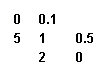 |
Note that empty spreadsheet cells (or cells containing non-numerical characters) represent the value 0 (zero). Now highlight the 3x3 matrix and select Math>Markov simulation>channels from the menu. A dialogue window will pop up requesting "timebase" (set this to 5 s), "number of sweeps" (leave this at 1 for the time being), "number of channels" (set this for example to 300) and "channels initially", (set this to "in state 1"). Click the "OK" button. A temporary file "serftmp.cha" is created. In the window that then appears, a name for the new data file may be chosen, which may not be "serftmp.cha" (it is not necessary to type the ".cha" extension, this will be added automatically if you have not done so).
Markov simulation>macroscopic current
The average behaviour of the transition matrix as the one shown above can be found with this menu item. First, the eigenvalues and eigenvectors of the matrix are calculated and then the initial conditions are used to scale the eigenvectors. The result will be a curve on the drawing sheet. Before using this menu item, select the square transition matrix, then select Math>Markov simulation>macroscopic current. A dialogue window comes up requesting the initial occupation of each state. Here, only positive numbers should be used. The interpretation of these numbers is up to the user; one might interpret these numbers as percentages and enter (for the model above) the values 100 for state number 1 and 0% for the remaining two, hence all channels start in state 1. In the edit box![]() "State" you'll find the values you've entered on the diagonal of the transition matrix (see: Markov simulation>channels) and that you may change here. Use the arrow buttons to move between state numbers. In "Timebase" choose the stretch of time you wish to simulate (in ms), Hence, timebase 500 will simulate half a second of channel activity. The "number of points" sets the number of data points that will appear in the graph. The amplitudes and the time constants of the exponentials composing the simulated current will be inserted onto the spreadsheet to the right of the transition matrix. If complex or repeated eigenvalues are found, the third column inserted, marked "*", will contain the function by which the exponential needs to be multiplied. Hence, if the result on a row reads "Amp:" 2, "-tau:" 3, "*:" sin(4t), then the resulting function is: 2*sin(4t)*exp(-t/3). Use the options "no graph", "on clipboard" or "new document" to have respectively: 1) no graph at all, 2) a graph resident on the clipboard that can subsequently be pasted onto a spreadsheet and/or a drawing sheet, or 3) a new drawing sheet containing the new histogram (the default).
"State" you'll find the values you've entered on the diagonal of the transition matrix (see: Markov simulation>channels) and that you may change here. Use the arrow buttons to move between state numbers. In "Timebase" choose the stretch of time you wish to simulate (in ms), Hence, timebase 500 will simulate half a second of channel activity. The "number of points" sets the number of data points that will appear in the graph. The amplitudes and the time constants of the exponentials composing the simulated current will be inserted onto the spreadsheet to the right of the transition matrix. If complex or repeated eigenvalues are found, the third column inserted, marked "*", will contain the function by which the exponential needs to be multiplied. Hence, if the result on a row reads "Amp:" 2, "-tau:" 3, "*:" sin(4t), then the resulting function is: 2*sin(4t)*exp(-t/3). Use the options "no graph", "on clipboard" or "new document" to have respectively: 1) no graph at all, 2) a graph resident on the clipboard that can subsequently be pasted onto a spreadsheet and/or a drawing sheet, or 3) a new drawing sheet containing the new histogram (the default).
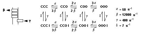
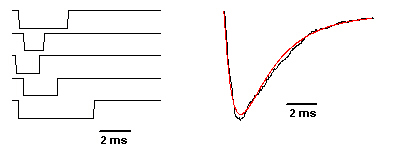
The figures underneath compare the results of the channels and the macroscopic current menu items, using the representation of the voltage-dependent sodium channel by Hodgkin and Huxley as an example. To the left in the figure is shown their mechanistic model of the channel containing 4 gates: 3 identical activation gates that, upon membrane depolarisation, open up with a rate constant β and a single inactivation gate that closes with a rate constant γ. The backward rate constants of these processes, α and δ respectively, are not shown in the figure. Their model can be transformed to a monomolecular reaction scheme as shown the middle, where 'CCO' means: two activation gates Closed and one activation gate Open. COOI means: one activation gate Closed, two activation gates Open and the channel Inactivated by closure of the Inactivation gate.
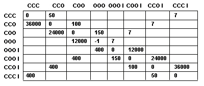
If the rate constants, corresponding to a depolarisation to +20 mV, are chosen as in the rightmost list, an 8*8 transition matrix can be constructed (the blank boxes representing zeros, which have been left out for clarity):
Five samples from a Markov simulation>channels simulation with one channel are shown underneath. The black line in the figure to the right shows the response of a Markov simulation>channels simulation with 1000 channels, while the red curve gives the result of the Markov simulation>macroscopic current simulation
In order to obtain the eigenvalues of the transition matrix using the Eigenvalues menu item, the state values on the diagonal need to be replaced by the correct rate constants corresponding to the 8 differential equations that govern the macroscopic current, i.e. the negative of the sum of rate constants over each column:
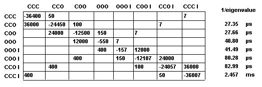
After execution of Eigenvalues, the relaxation rate constants (eigenvalues) are found. The seven time constants (1/rate constant) are shown to the right in the figure above. UP↑
Markov simulation>Open/Closed times
The time constants and amplitudes of the exponentials describing the open time or closed time distributions associated with the Markov transition matrix can be found using this menu item. In the dialogue that pops up, select either "open time" or "closed time". Select next whether the open/closed time distribution should be constructed with the system in equilibrium or off-equilibrium. In the latter case, enter the occupation of each of the states as described in the Macroscopic current section above. The calibration of the Y axis is calculated in such a way that the total surface of the distribution amounts to P = 1. Hence, the data points in the graph represent probability density, which may be expressed either as probability per second or probability per bin. The bin width is determined by the quotient of the entries in "Timebase" and "# points in graph". After calculation, the time constants and amplitudes of the exponentials will be inserted onto the spreadsheet to the right of the transition matrix. If complex or repeated eigenvalues are found, the third column inserted, marked "*", will contain the function by which the exponential needs to be multiplied. Hence, if the result on a row reads "Amp:" 2, "-tau:" 3, "*:" sin(4t), then the resulting function is: 2*sin(4t)*exp(-t/3). Use the options "no graph", "on clipboard" or "new document" to have respectively: 1) no graph at all, 2) a graph resident on the clipboard that can subsequently be pasted onto a spreadsheet and/or a drawing sheet, or 3) a new drawing sheet containing the new histogram (the default).
Markov simulation>First latency
The time constants and amplitudes of the exponentials describing the first latency distribution associated with the Markov transition matrix can be found using this menu item. In the dialogue that pops up, select whether the first latency distribution should be constructed with the system in equilibrium or off-equilibrium. In the latter case, enter the occupation of each of the states as described in the Macroscopic current section above. The calibration of the Y axis is calculated in such a way that the total surface of the distribution amounts to P = 1. Hence, the data points in the graph represent probability density, which may be expressed either as probability per second or probability per bin. The bin width is determined by the quotient of the entries in "Timebase" and "# points in graph". After calculation, the time constants and amplitudes of the exponentials will be inserted onto the spreadsheet to the right of the transition matrix. If complex or repeated eigenvalues are found, the third column inserted, marked "*", will contain the function by which the exponential needs to be multiplied. Hence if the result on a row reads "Amp:" 2, "-tau:" 3, "*:" t, then the resulting function is: 2*t*exp(-t/3). Use the options "no graph", "on clipboard" or "new document" to have respectively: 1) no graph at all, 2) a graph resident on the clipboard that can subsequently be pasted onto a spreadsheet and/or a drawing sheet, or 3) a new drawing sheet containing the new histogram (the default).UP↑
Markov simulation>Fit rate constants
Given a model (i.e. a Markov chain in this context), then the rate constants of the model in question may be estimated from experimental data (i.e. macroscopic current, first latency and open/closed time distributions). Before issuing the Fit rate constants command, make sure that the very same spreadsheet contains both a transition matrix and experimental data. The latter should be organised in columns. A column (Y-column) containing macroscopic current or dwell time distribution data must be preceeded by a column (X-column) with its timebase. A single X-column may do for several Y-columns that follow it. The time base should be in seconds ("s") unless the uppermost cell contains the text: "ms" (milliseconds), "μs" (microseconds) or "min" (minutes). In that case, the appropriate conversion into seconds is carried out automatically and the X-column is replaced by one reading the timebase in seconds. The transition matrix should contain zeroes or blanks (0) and ones (1) in the diagonal elements, indicating closed (0) and open (1) states. Off-diagonal elements containing non-zero values will be used as first estimates for the rate constants to fit. Elements left blank or containing zeroes are ignored (i.e. will not be fitted) and are considered to have zero transition probability all along. A valid spreadsheet entry is shown in the example below:
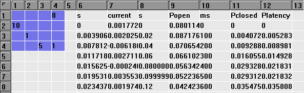
In the figure the spreadsheet shows only the upper 8 cells. In fact columns 6 & 7 have 501 cells, while the following columns each have 51 cells, including the headers. Columns 11 & 12 use the same timebase in column 10. The 4x4 transition matrix is highlighted in blue, indicating one open state (state 4) and 4 rate constants to fit.
After having highlighted the transition matrix and having issued the Fit rate constants command, a dialogue window pops up:
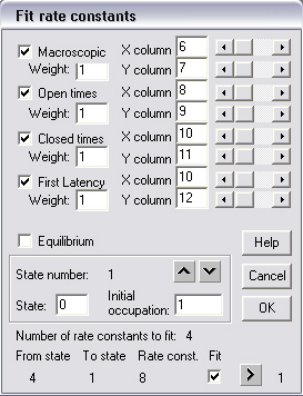 Check the "Macroscopic" (macroscopic current), "Open times", "Closed times" and "First latency" checkboxes if the spreadsheet contains data thereof, which is the case here. Enter the X (timebase) and Y (current, probabilities) spreadsheet columns in the edit box
![]() es marked by "X column" and "Y column" respectively. The edit box
es marked by "X column" and "Y column" respectively. The edit box![]() entries can also be set using the slide bars to the right. In this example, the first latency data are in spreadsheet columns 10 and 12. Set the values in the "Weight" edit box
entries can also be set using the slide bars to the right. In this example, the first latency data are in spreadsheet columns 10 and 12. Set the values in the "Weight" edit box![]() es to indicate the importance of the experimental data. If the data in question is not very reliable, choose a value below 1. Valid entries are between 0.01 and 100.
If the spreadsheet data was obtained with channel activity in equilibrium, check the "Equilibrium" check box. If not, set for each state number (here 1 through 4) the initial occupation of the states in arbitrary units (the sum will be normalised to 1 afterwards). Use the
es to indicate the importance of the experimental data. If the data in question is not very reliable, choose a value below 1. Valid entries are between 0.01 and 100.
If the spreadsheet data was obtained with channel activity in equilibrium, check the "Equilibrium" check box. If not, set for each state number (here 1 through 4) the initial occupation of the states in arbitrary units (the sum will be normalised to 1 afterwards). Use the ![]() and
and ![]() buttons to shift through state numbers.
The lower part of the dialogue box enumerates the rate constants to fit. Per default, all rate constants (that is to say, those different from zero) will be fit. If one wishes to fix one of the rate constants, uncheck the "Fit" checkbox for that rate constant. Use the
buttons to shift through state numbers.
The lower part of the dialogue box enumerates the rate constants to fit. Per default, all rate constants (that is to say, those different from zero) will be fit. If one wishes to fix one of the rate constants, uncheck the "Fit" checkbox for that rate constant. Use the ![]() button to go to the next rate constant.
button to go to the next rate constant.
Once all is done, push the "OK" button.
After a few hundred iterations the transition matrix on the spreadsheet is updated with estimations of the rate constants and underneath it, two lines indicate the (mean) square difference of experimental and calculated data points (marked "SSQ") and the number of iterations that was required. If the latter equals or exceeds 2000, the fit routine has possibly ended without reaching conversion. It is not a bad idea to refit the data with the newly found rate constants as first estimates to see whether SSQ remains stable.UP↑
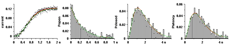
The data in the example above has been generated using the Markov simulation>macroscopic current, Markov simulation>Open/Closed times and Markov simulation>First latency commands using the transition matrix if the figure below (A). Gauss-distributed noise was added and the rate constants were fitted using the matrix in B as initial estimates. This resulted in matrix C, which differs from from the original in A.
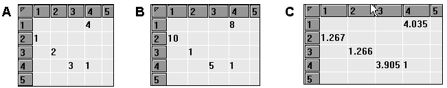
However, when plotting the data (red curves: distributions calculated with matrix A; black points and bars: the same distributions to which noise was added) and estimates (green curves: distributions calculated with matrix C), the fit is almost perfect. This is due to the fact that the representation in A is not a unique solution. For example, the rate constants with the values 1,2 and 3 can obviously appear in any order without changing the resulting distributions. The lack of uniqueness may pose a problem of interpretation that the user should be aware of when comparing results.
Eigenvalues
Eigenvalues are a special set of values associated with a linear system of equations (i.e., a matrix equation) that are sometimes also known as characteristic roots, proper values, or latent roots. The determination of the eigenvalues and eigenvectors of a system is extremely important in physics and engineering, where it is equivalent to matrix diagonalisation and arises in such common applications as the physics of rotating bodies, and small oscillations of vibrating systems, to name only two. Each eigenvalue is paired with a corresponding so-called eigenvector. The decomposition of a square matrix into eigenvalues and eigenvectors is known as eigen decomposition, and the fact that this decomposition is always possible as long a the matrix consisting of the eigenvectors is square is known as the eigen decomposition theorem. Let A be a linear transformation represented by a matrix A. If there is a vector X such that AX = eX for some scalar e, then e is called the eigenvalue of A with corresponding eigenvector X. The program uses a method known as the double step implicit QR algorithm to carry out the eigen decomposition. It almost always finds the eigenvalues, but it has some limitations regarding the determination of eigenvectors: it does not calculate eigenvectors associated with multiple repeated real roots having mixed dependent and independent eigenvectors and it does not calculate eigenvectors associated with repeated complex roots, as these events seem to be too rare to make them worth the programming effort. However, if this turns out to be a problem, drop a line at serf-at-bram.org.
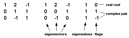
To calculate the eigenvalues of a square matrix, select the range of spreadsheet cells that contains the N*N matrix and then select this menu item. Make sure that the dimensions (N lines and N columns) are correct. If not, an error message will be issued. Upon return of the algorithm, a N*N matrix containing the eigenvectors will be pasted on the spreadsheet to the right of the original matrix. This matrix is followed by two columns; the first contains the eigenvalues and the second contains flags signalling the properties of the eigenvalues. Eigenvectors and eigenvalues are listed in the same order, i.e. the leftmost vector corresponds to the first eigenvalue etc. Flag 0 indicates an isolated real root. Flag 1 indicates the real part of a complex root. Flag -1 indicates the imaginary part of a complex root. The flags 1 and -1 always appear in pairs. Flag 2 indicates a repeated real root with dependent vectors. The second repeated root, also flagged 2, immediately follows the first one. Repeated roots with independent vectors are flagged 0, as for isolated roots. Flag 3 indicates that convergence for this root has not been obtained and that the result is probably incorrect.
In the example underneath, a 3*3 matrix yields 1 real eigenvalue (1) and a pair of complex eigenvalues (1+i and 1-i).
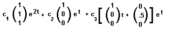
Therefore the solution of the three differential equations to the left is:
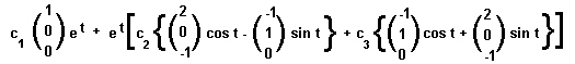
where the constants c1, c2 and c3 will be determined by the boundary conditions.
In the next example, two repeated roots are found:
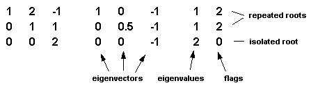
As the repeated roots are flagged 2, the first two vectors are dependent and the above result (after multiplication of the isolated vector by -1) should be interpreted as follows:
 UP↑
UP↑
Covariance matrix
The Covariance, Cov(x,y), of two columns of data x and y of lengths n is given by:
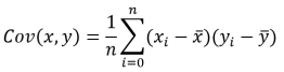
The m*m covariance matrix, C, describes the covariance of each of the m vectors (columns) of length n in a n*m matrix, M, with the other vectors in that matrix. The elements on the diagonal of the covariance matrix correspond to the covariance of a vector with itself, hence it is its variance. The covariance matrix is symmetrical across its diagonal since Cov(Vi,Vj) = Cov(Vj,Vi).
The eigen decomposition of the covariance matrix gives a set of orthogonal vectors that contain the principal components of matrix M. These components are used in Principal Component Analysis (PCA).
Correlation matrix
The Pearson correlation coefficient of two vectors, x and y is:
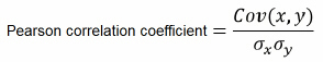
where σx and σy are the standard deviations of the data in columns x and y (i.e. the square root of the variance).The correlation matrix is obtained from the covariance matrix using this equation. In concreto, by dividing each element C[i,j] by the square root of the product of the diagonal elements C[i,i]*C[j,j].
Principle component analysis
Select a rectangle of data (hence not columns this time) prior to execute the Principal component analysis (PCA) command. The program then calculates the covariance matrix and shows the variances associated with each column vector. Next it shows the eigenvectors and eigenvalues of the covariance matrix. These are then used to calculate the components (columns), which are shown in decreasing order with respect to the variance they represent (shown underneath the components). Next a dialogue window pops up asking for the number of principal components to use for the reconstruction of the original data. This last step serves to confirm that the first PCs chosen are actually enough to represent the original data reliably.
3 PC Graph
Select a rectangle of data (matrix) as in the previous sections. The program will then create a 3D Graph showing the three principal components of the original matrix.UP↑
Spreadsheet functions
Calculations
The operators for addition '+', subtraction '-', multiplication '*', division '/' and raising to a power '**' or '^' should be used respecting the normal rules for commutation (e.g. 2+3 is the same as 3+2), association (e.g. 2*(3*5) is the same as (2*3)*5) and distribution (e.g. 2*5+3*5 is the same as (2+3)*5). If in doubt, use brackets.
Raising the power takes precedence over the other operators. Multiplicatiopn and division take precedence over addition and subtraction (e.g. 2+3/5 is the same as 2+(3/5) and is not the same as (2+3)/5).
|Function list| UP↑
Boolean operations
Boolean operations are carried out between variables that have only two states: true (1) or false (0). Comparisons in the next section return a boolean. This program knows three operations AND (or &, as in the C language), OR (or |, as in C), and NOT (or ~, as in formal logic notation.
The notation is as for addition and multiplication, e.g. 1 AND 0.
0 AND 0 = 0 0 OR 0 = 0
1 AND 0 = 0 1 OR 0 = 1
1 AND 1 = 1 1 OR 1 = 1
NOT 1 = 0
NOT 0 = 1
|Function list| UP↑
Comparisons
With the operators '<', '≤', '=', '≥' et '>' numbers may be compared. The result is a boolean (1 or 0, true or false, yes or no).
1>2 gives 0, 300>=56 gives 1
Multiple comparisons can be combined using brackets and boolean operators: (1>12) OR (300≥56) gives 1.
|Function list| UP↑
CIN
Cin does not take arguments and returns the column number in which 'cin' finds itself. This function can be used in calculations: e.g. Cell(cin+6;3), which means "take the contents of the cell that is on the current line but is 6 columns farther away".
|Function list| UP↑
LIN
Lin does not take arguments and returns the line number in which 'lin' finds itself. This function can be used in calculations: e.g. Cell(3;lin+6), which means "take the contents of the cell that is in the current column but is 6 lines downward".
|Function list| UP↑
CELL
Cell(c;l) returns the numerical value of the spreadsheet cell at column c and line l. If the cell contains text, if the cell is empty or if the formula it contains is erroneous, the function returns 0 (zero). Cell( ) differs from a spreadsheet cell reference (e.g. (C1:L2) ) in that it's arguments may be references or the result of a calculation or a Boolean expression (e.g. Cell(sqr(4);(C1:L2)>1) ).
|Function list| UP↑
SUM
Sum(range) takes the sum of a range of cells.
There are two ways to enter a range in a function:
i) Type it (e.g. "sum(C2:L2;C2:L300)"), N.B.: do not type the quotation characters, or
ii) in the spreadsheet edit box![]() type "=sum(" and place the cursor behind the bracket "(". Then right-button-click the first cell of the range in the spreadsheet and move the mouse while keeping the right mouse button depressed. Release the mouse button at the last cell to be included. The range selected for the function appears in the edit box
type "=sum(" and place the cursor behind the bracket "(". Then right-button-click the first cell of the range in the spreadsheet and move the mouse while keeping the right mouse button depressed. Release the mouse button at the last cell to be included. The range selected for the function appears in the edit box![]() , the closing bracket ")" is added and the corresponding cells in the spreadsheet are highlighted in yellow.
, the closing bracket ")" is added and the corresponding cells in the spreadsheet are highlighted in yellow.
The conditional form of this function takes a condition as a second parameter and a third parameter that indicates the upper left spreadsheet cell of a range of cells with the same dimensions as the first range of cells. Thus, to each cell in the first range corresponds a cell in the second range. If the content of the cell in the second range satisfies the condition, then the content of the cell in the first is taken into account by the function. The condition consists of one of the operators =, >, <, ≥ or ≤ followed by a (floating point) number.
The syntax is Sum((range);condition;[cell]).
|Function list| UP↑
AVERAGE or MEAN
Average(range) and mean(range) calculate the average value of a range of cells.
There are two ways to enter a range in a function:
i) Type it (e.g. "mean(C2:L2;C2:L300)"), N.B.: do not type the quotation characters, or
ii) in the spreadsheet edit box![]() type "=mean(" and place the cursor behind the bracket "(". Then right-button-click the first cell of the range in the spreadsheet and move the mouse while keeping the right mouse button depressed. Release the mouse button at the last cell to be included. The range selected for the function appears in the edit box
type "=mean(" and place the cursor behind the bracket "(". Then right-button-click the first cell of the range in the spreadsheet and move the mouse while keeping the right mouse button depressed. Release the mouse button at the last cell to be included. The range selected for the function appears in the edit box![]() , the closing bracket ")" is added and the corresponding cells in the spreadsheet are highlighted in yellow.
, the closing bracket ")" is added and the corresponding cells in the spreadsheet are highlighted in yellow.
The conditional form of this function takes a condition as a second parameter and a third parameter that indicates the upper left spreadsheet cell of a range of cells with the same dimensions as the first range of cells. Thus, to each cell in the first range corresponds a cell in the second range. If the content of the cell in the second range satisfies the condition, then the content of the cell in the first is taken into account by the function. The condition consists of one of the operators =, >, <, ≥ or ≤ followed by a (floating point) number.
The syntax is Average((range); condition;[cell]).
|Function list| UP↑
STDEV
Stdev(range) calculates the standard deviation of a range of cells. It assumes a Gaussian probability distribution. See also SEM( ).
There are two ways to enter a range in a function:
i) Type it (e.g. "stdev(C2:L2;C2:L300)"), N.B.: do not type the quotation characters, or
ii) in the spreadsheet edit box![]() type "=stdev(" and place the cursor behind the bracket "(". Then right-button-click the first cell of the range in the spreadsheet and move the mouse while keeping the right mouse button depressed. Release the mouse button at the last cell to be included. The range selected for the function appears in the edit box
type "=stdev(" and place the cursor behind the bracket "(". Then right-button-click the first cell of the range in the spreadsheet and move the mouse while keeping the right mouse button depressed. Release the mouse button at the last cell to be included. The range selected for the function appears in the edit box![]() , the closing bracket ")" is added and the corresponding cells in the spreadsheet are highlighted in yellow.
, the closing bracket ")" is added and the corresponding cells in the spreadsheet are highlighted in yellow.
The conditional form of this function takes a condition as a second parameter and a third parameter that indicates the upper left spreadsheet cell of a range of cells with the same dimensions as the first range of cells. Thus, to each cell in the first range corresponds a cell in the second range. If the content of the cell in the second range satisfies the condition, then the content of the cell in the first is taken into account by the function. The condition consists of one of the operators =, >, <, ≥ or ≤ followed by a (floating point) number.
The syntax is Stdev((range); condition;[cell]).
|Function list| UP↑
SEM
Sem(range) calculates the standard error of the mean of a range of cells. It assumes a Gaussian probability distribution. See also STDEV.
There are two ways to enter a range in a function:
i) Type it (e.g. "sem(C2:L2;C2:L300)"), N.B.: do not type the quotation characters, or
ii) in the spreadsheet edit box![]() type "=sem(" and place the cursor behind the bracket "(". Then right-button-click the first cell of the range in the spreadsheet and move the mouse while keeping the right mouse button depressed. Release the mouse button at the last cell to be included. The range selected for the function appears in the edit box
type "=sem(" and place the cursor behind the bracket "(". Then right-button-click the first cell of the range in the spreadsheet and move the mouse while keeping the right mouse button depressed. Release the mouse button at the last cell to be included. The range selected for the function appears in the edit box![]() , the closing bracket ")" is added and the corresponding cells in the spreadsheet are highlighted in yellow.
, the closing bracket ")" is added and the corresponding cells in the spreadsheet are highlighted in yellow.
The conditional form of this function takes a condition as a second parameter and a third parameter that indicates the upper left spreadsheet cell of a range of cells with the same dimensions as the first range of cells. Thus, to each cell in the first range corresponds a cell in the second range. If the content of the cell in the second range satisfies the condition, then the content of the cell in the first is taken into account by the function. The condition consists of one of the operators =, >, <, ≥ or ≤ followed by a (floating point) number.
The syntax is Sem((range); condition;[cell]).
|Function list| UP↑
MIN
Min(range) retrieves the minimum value of a range of cells. To retrieve the row and column indices of the cell containing the minimum value use the LIMIN( ) and CIMIN( ) functions respectively.
There are two ways to enter a range in a function:
i) Type it (e.g. "min(C2:L2;C2:L300)"), N.B.: do not type the quotation characters, or
ii) in the spreadsheet edit box![]() type "=min(" and place the cursor behind the bracket "(". Then right-button-click the first cell of the range in the spreadsheet and move the mouse while keeping the right mouse button depressed. Release the mouse button at the last cell to be included. The range selected for the function appears in the edit box
type "=min(" and place the cursor behind the bracket "(". Then right-button-click the first cell of the range in the spreadsheet and move the mouse while keeping the right mouse button depressed. Release the mouse button at the last cell to be included. The range selected for the function appears in the edit box![]() , the closing bracket ")" is added and the corresponding cells in the spreadsheet are highlighted in yellow.
, the closing bracket ")" is added and the corresponding cells in the spreadsheet are highlighted in yellow.
The conditional form of this function takes a condition as a second parameter and a third parameter that indicates the upper left spreadsheet cell of a range of cells with the same dimensions as the first range of cells. Thus, to each cell in the first range corresponds a cell in the second range. If the content of the cell in the second range satisfies the condition, then the content of the cell in the first is taken into account by the function. The condition consists of one of the operators =, >, <, ≥ or ≤ followed by a (floating point) number.
The syntax is Min((range); condition;[cell])
|Function list| UP↑
MAX
Max(range) retrieves the maximum value of a range of cells. To retrieve the row and column indices of the cell containing the maximum value use the LIMAX( ) and CIMAX( ) functions respectively.
There are two ways to enter a range in a function:
i) Type it (e.g. "max(C2:L2;C2:L300)"), N.B.: do not type the quotation characters, or
ii) in the spreadsheet edit box![]() type "=max(" and place the cursor behind the bracket "(". Then right-button-click the first cell of the range in the spreadsheet and move the mouse while keeping the right mouse button depressed. Release the mouse button at the last cell to be included. The range selected for the function appears in the edit box
type "=max(" and place the cursor behind the bracket "(". Then right-button-click the first cell of the range in the spreadsheet and move the mouse while keeping the right mouse button depressed. Release the mouse button at the last cell to be included. The range selected for the function appears in the edit box![]() , the closing bracket ")" is added and the corresponding cells in the spreadsheet are highlighted in yellow.
, the closing bracket ")" is added and the corresponding cells in the spreadsheet are highlighted in yellow.
The conditional form of this function takes a condition as a second parameter and a third parameter that indicates the upper left spreadsheet cell of a range of cells with the same dimensions as the first range of cells. Thus, to each cell in the first range corresponds a cell in the second range. If the content of the cell in the second range satisfies the condition, then the content of the cell in the first is taken into account by the function. The condition consists of one of the operators =, >, <, ≥ or ≤ followed by a (floating point) number.
The syntax is Max((range); condition;[cell])
|Function list| UP↑
SQR or SQRT
Sqrt(x) and sqr(x) return the square root of x (e.g. =sqr(4) returns 2).
Domain: all v>0. Hence sqr(-3) will return a domain error message.
This function only demands a single parameter. If you wish this parameter to be a reference rather than a number, type for instance "=sqr[C2:L3]". A second way to enter the reference is the following: in the edit box![]() type "=sqr", then right-button click the spreadsheet cell that contains the argument. The text string will then read: "=sqr[Cn:Lm]", where n and m are the indices of the cell containing the argument.
type "=sqr", then right-button click the spreadsheet cell that contains the argument. The text string will then read: "=sqr[Cn:Lm]", where n and m are the indices of the cell containing the argument.
|Function list| UP↑
SIN
Sin(x) returns the sine of x, where x is in radians.
This function only demands a single parameter. If you wish this parameter to be a reference rather than a number, type for instance "=sin[C2:L3]". A second way to enter the reference is the following: in the edit box![]() type "=sin", then right-button click the spreadsheet cell that contains the argument. The text string will then read: "=sin[Cn:Lm]", where n and m are the indices of the cell containing the argument.
type "=sin", then right-button click the spreadsheet cell that contains the argument. The text string will then read: "=sin[Cn:Lm]", where n and m are the indices of the cell containing the argument.
|Function list| UP↑
COS
Cos(x) returns the cosine of x, where x is in radians.
This function only demands a single parameter. If you wish this parameter to be a reference rather than a number, type for instance "=cos[C2:L3]". A second way to enter the reference is the following: in the edit box![]() type "=cos", then right-button click the spreadsheet cell that contains the argument. The text string will then read: "=cos[Cn:Lm]", where n and m are the indices of the cell containing the argument.
type "=cos", then right-button click the spreadsheet cell that contains the argument. The text string will then read: "=cos[Cn:Lm]", where n and m are the indices of the cell containing the argument.
|Function list| UP↑
TAN
Tan(x) returns the tangent of x, where x is in radians. To obtain the cotangent enter "=1/tan(x)".
This function only demands a single parameter. If you wish this parameter to be a reference rather than a number, type for instance "=tan[C2:L3]". A second way to enter the reference is the following: in the edit box![]() type "=tan", then right-button click the spreadsheet cell that contains the argument. The text string will then read: "=tan[Cn:Lm]", where n and m are the indices of the cell containing the argument.
type "=tan", then right-button click the spreadsheet cell that contains the argument. The text string will then read: "=tan[Cn:Lm]", where n and m are the indices of the cell containing the argument.
|Function list| UP↑
ASIN
Asin(x) calculates the arcsine of x, returning the angle in radians.
This function only demands a single parameter. If you wish this parameter to be a reference rather than a number, type for instance "=asin[C2:L3]". A second way to enter the reference is the following: in the edit box![]() type "=asin", then right-button click the spreadsheet cell that contains the argument. The text string will then read: "=asin[Cn:Lm]", where n and m are the indices of the cell containing the argument.
type "=asin", then right-button click the spreadsheet cell that contains the argument. The text string will then read: "=asin[Cn:Lm]", where n and m are the indices of the cell containing the argument.
Domain: -1 <= x <= 1
|Function list| UP↑
ACOS
Acos(x) calculates the arccosine of x, returning the angle in radians.
This function only demands a single parameter. If you wish this parameter to be a reference rather than a number, type for instance "=acos[C2:L3]". A second way to enter the reference is the following: in the edit box![]() type "= acos", then right-button click the spreadsheet cell that contains the argument. The text string will then read: "= acos[Cn:Lm]", where n and m are the indices of the cell containing the argument.
type "= acos", then right-button click the spreadsheet cell that contains the argument. The text string will then read: "= acos[Cn:Lm]", where n and m are the indices of the cell containing the argument.
Domain: -1 <= x <= 1
|Function list| UP↑
ATAN
Atan(x) calculates the arctangent of x, returning the angle in radians. To obtain the arccotangent enter "=atan(1/x)".
This function only demands a single parameter. If you wish this parameter to be a reference rather than a number, type for instance "=atan[C2:L3]". A second way to enter the reference is the following: in the edit box![]() type "= atan", then right-button click the spreadsheet cell that contains the argument. The text string will then read: "= atan[Cn:Lm]", where n and m are the indices of the cell containing the argument.
type "= atan", then right-button click the spreadsheet cell that contains the argument. The text string will then read: "= atan[Cn:Lm]", where n and m are the indices of the cell containing the argument.
|Function list| UP↑
LN
Ln(x) returns the natural logarithm of x. It is the inverse of the EXP( ) function. See LOG( ) for the decimal logarithm.
Domain: all x>0.
This function only demands a single parameter. If you wish this parameter to be a reference rather than a number, type for instance "=ln[C2:L3]". A second way to enter the reference is the following: in the edit box![]() type "=ln", then right-button click the spreadsheet cell that contains the argument. The text string will then read: "=ln[Cn:Lm]", where n and m are the indices of the cell containing the argument.
type "=ln", then right-button click the spreadsheet cell that contains the argument. The text string will then read: "=ln[Cn:Lm]", where n and m are the indices of the cell containing the argument.
|Function list| UP↑
LOG
Log(x) returns the decimal logarithm of x. It is the inverse of 10**x (10 to the power of x). See LN( ) for the natural logarithm.
Domain: all x>0.
This function only demands a single parameter. If you wish this parameter to be a reference rather than a number, type for instance "=log[C2:L3]". A second way to enter the reference is the following: in the edit box![]() type "=log", then right-button click the spreadsheet cell that contains the argument. The text string will then read: "=log[Cn:Lm]", where n and m are the indices of the cell containing the argument.
type "=log", then right-button click the spreadsheet cell that contains the argument. The text string will then read: "=log[Cn:Lm]", where n and m are the indices of the cell containing the argument.
|Function list| UP↑
EXP
Exp(x) returns the exponential of x, e**x.
Domain: all x<76. For x>75 the function returns an error message.
This function only demands a single parameter. If you wish this parameter to be a reference rather than a number, type for instance "=exp[C2:L3]". A second way to enter the reference is the following: in the edit box![]() type "=exp", then right-button click the spreadsheet cell that contains the argument. The text string will then read: "=exp[Cn:Lm]", where n and m are the indices of the cell containing the argument.
type "=exp", then right-button click the spreadsheet cell that contains the argument. The text string will then read: "=exp[Cn:Lm]", where n and m are the indices of the cell containing the argument.
|Function list| UP↑
SIGN
Sign(x) returns -1 for x<0 and +1 for x>=0.
This function only demands a single parameter. If you wish this parameter to be a reference rather than a number, type for instance "=sign[C2:L3]". A second way to enter the reference is the following: in the edit box![]() type "=sign", then right-button click the spreadsheet cell that contains the argument. The text string will then read: "=sign[Cn:Lm]", where n and m are the indices of the cell containing the argument.
type "=sign", then right-button click the spreadsheet cell that contains the argument. The text string will then read: "=sign[Cn:Lm]", where n and m are the indices of the cell containing the argument.
|Function list| UP↑
ABS
Abs(x) returns the absolute value of x. Hence abs(-6.3) gives 6.3.
This function only demands a single parameter. If you wish this parameter to be a reference rather than a number, type for instance "=abs[C2:L3]". A second way to enter the reference is the following: in the edit box![]() type "=abs", then right-button click the spreadsheet cell that contains the argument. The text string will then read: "=abs[Cn:Lm]", where n and m are the indices of the cell containing the argument.
type "=abs", then right-button click the spreadsheet cell that contains the argument. The text string will then read: "=abs[Cn:Lm]", where n and m are the indices of the cell containing the argument.
|Function list| UP↑
INT
Int(x) truncates x to an integer value. Hence int(5.7) gives 5.
This function only demands a single parameter. If you wish this parameter to be a reference rather than a number, type for instance "=int[C2:L3]". A second way to enter the reference is the following: in the edit box![]() type "=int", then right-button click the spreadsheet cell that contains the argument. The text string will then read: "=int[Cn:Lm]", where n and m are the indices of the cell containing the argument.
type "=int", then right-button click the spreadsheet cell that contains the argument. The text string will then read: "=int[Cn:Lm]", where n and m are the indices of the cell containing the argument.
|Function list| UP↑
BINOM
Binom(N;k) returns the coefficient of the k'th term of an N-binomial. The coefficients of the terms may be found by expanding "Pascal's triangle":
N=0 1
1 1 1
2 1 2 1
3 1 3 3 1
4 1 4 6 4 1 etc,
The numbers in each new row are the sum of the two numbers just above, adding 1s at the borders. The coefficients may also be calculated using the formula:
ck = N! / ( k! . (N-k)! )
Note that both N and k start at 0. Hence binom(3;0) = 1 and the 2nd term (k=1) of a 4 binomial (n=4) equals 4. Binom(4;2)=6 etc. |Function list| UP↑
CHIDIST
Chidist(c2;df) returns the probability of a chi-2 value at df degrees of freedom.
Chidist(c2;df) is used to find the statistical probability of the outcome the chi-square test.

|Function list| UP↑
TDIST
Tdist(t;df;s) returns the probability of a t-value at df degrees of freedom, single sided (s=1) or double sided (s=2). It is the integral of TDENS( ). Tval(p;df;s) is its inverse function (i.e. it returns the t-value, given the probability p, df and s).
Tdist is used to find the statistical probability of the outcome of Student's t-test. A Gaussian distribution is assumed.
Domain: t>0 & df>0

|Function list| UP↑
RAND
Rand(x) returns a random floating point number between 0 and x. The outcome of all values between 0 and x have equal probability.
|Function list| UP↑
CIMIN
Cimin(range) returns the column index of the spreadsheet cell containing the minimum in the range of cells. To obtain the minimum value itself use the MIN( ) function.
There are two ways to enter a range in a function:
i) Type it (e.g. "cimin(C2:L2;C2:L300)"), N.B.: do not type the quotation characters, or
ii) in the spreadsheet edit box![]() type "=cimin(" and place the cursor behind the bracket "(". Then right-button-click the first cell of the range in the spreadsheet and move the mouse while keeping the right mouse button depressed. Release the mouse button at the last cell to be included. The range selected for the function appears in the edit box
type "=cimin(" and place the cursor behind the bracket "(". Then right-button-click the first cell of the range in the spreadsheet and move the mouse while keeping the right mouse button depressed. Release the mouse button at the last cell to be included. The range selected for the function appears in the edit box![]() , the closing bracket ")" is added and the corresponding cells in the spreadsheet are highlighted in yellow.
, the closing bracket ")" is added and the corresponding cells in the spreadsheet are highlighted in yellow.
The conditional form of this function takes a condition as a second parameter and a third parameter that indicates the upper left spreadsheet cell of a range of cells with the same dimensions as the first range of cells. Thus, to each cell in the first range corresponds a cell in the second range. If the content of the cell in the second range satisfies the condition, then the content of the cell in the first is taken into account by the function. The condition consists of one of the operators =, >, ≤, > or ≥ followed by a (floating point) number.
The syntax is Cimin((range); condition;[cell]).
|Function list| UP↑
CIMAX
Cimax(range) returns the column index of the spreadsheet cell containing the maximum in the range of cells. To obtain the maximum value itself use the MAX( ) function.
There are two ways to enter a range in a function:
i) Type it (e.g. "cimax(C2:L2;C2:L300)"), N.B.: do not type the quotation characters, or
ii) in the spreadsheet edit box![]() type "=cimax(" and place the cursor behind the bracket "(". Then right-button-click the first cell of the range in the spreadsheet and move the mouse while keeping the right mouse button depressed. Release the mouse button at the last cell to be included. The range selected for the function appears in the edit box
type "=cimax(" and place the cursor behind the bracket "(". Then right-button-click the first cell of the range in the spreadsheet and move the mouse while keeping the right mouse button depressed. Release the mouse button at the last cell to be included. The range selected for the function appears in the edit box![]() , the closing bracket ")" is added and the corresponding cells in the spreadsheet are highlighted in yellow.
, the closing bracket ")" is added and the corresponding cells in the spreadsheet are highlighted in yellow.
The conditional form of this function takes a condition as a second parameter and a third parameter that indicates the upper left spreadsheet cell of a range of cells with the same dimensions as the first range of cells. Thus, to each cell in the first range corresponds a cell in the second range. If the content of the cell in the second range satisfies the condition, then the content of the cell in the first is taken into account by the function. The condition consists of one of the operators =, >, ≤, > or ≥ followed by a (floating point) number.
The syntax is Cimax((range); condition;[cell])
|Function list| UP↑
LIMIN
Limin(range) returns the line (row) index of the spreadsheet cell containing the minimum in the range of cells. To obtain the minimum value itself use the MIN( ) function.
There are two ways to enter a range in a function:
i) Type it (e.g. "limin(C2:L2;C2:L300)"), N.B.: do not type the quotation characters, or
ii) in the spreadsheet edit box![]() type "=limin(" and place the cursor behind the bracket "(". Then right-button-click the first cell of the range in the spreadsheet and move the mouse while keeping the right mouse button depressed. Release the mouse button at the last cell to be included. The range selected for the function appears in the edit box
type "=limin(" and place the cursor behind the bracket "(". Then right-button-click the first cell of the range in the spreadsheet and move the mouse while keeping the right mouse button depressed. Release the mouse button at the last cell to be included. The range selected for the function appears in the edit box![]() , the closing bracket ")" is added and the corresponding cells in the spreadsheet are highlighted in yellow.
, the closing bracket ")" is added and the corresponding cells in the spreadsheet are highlighted in yellow.
The conditional form of this function takes a condition as a second parameter and a third parameter that indicates the upper left spreadsheet cell of a range of cells with the same dimensions as the first range of cells. Thus, to each cell in the first range corresponds a cell in the second range. If the content of the cell in the second range satisfies the condition, then the content of the cell in the first is taken into account by the function. The condition consists of one of the operators =, >, ≤, > or ≥ followed by a (floating point) number.
The syntax is Limin((range); condition;[cell])
|Function list| UP↑
LIMAX
Limax(range) returns the line (row) index of the spreadsheet cell containing the maximum in the range of cells. To obtain the maximum value itself use the MAX( ) function.
There are two ways to enter a range in a function:
i) Type it (e.g. "limax(C2:L2;C2:L300)"), N.B.: do not type the quotation characters, or
ii) in the spreadsheet edit box![]() type "=limax(" and place the cursor behind the bracket "(". Then right-button-click the first cell of the range in the spreadsheet and move the mouse while keeping the right mouse button depressed. Release the mouse button at the last cell to be included. The range selected for the function appears in the edit box
type "=limax(" and place the cursor behind the bracket "(". Then right-button-click the first cell of the range in the spreadsheet and move the mouse while keeping the right mouse button depressed. Release the mouse button at the last cell to be included. The range selected for the function appears in the edit box![]() , the closing bracket ")" is added and the corresponding cells in the spreadsheet are highlighted in yellow.
, the closing bracket ")" is added and the corresponding cells in the spreadsheet are highlighted in yellow.
The conditional form of this function takes a condition as a second parameter and a third parameter that indicates the upper left spreadsheet cell of a range of cells with the same dimensions as the first range of cells. Thus, to each cell in the first range corresponds a cell in the second range. If the content of the cell in the second range satisfies the condition, then the content of the cell in the first is taken into account by the function. The condition consists of one of the operators =, >, ≤, > or ≥ followed by a (floating point) number.
The syntax is Limax((range); condition;[cell]).
|Function list| UP↑
TIME
Time(h,m,s) takes three parameters h (hours), m (minutes) and s (seconds) and returns the "time" format: "h:m:s". h,m and s may be floating point. Hence "=time(1.5;0;0)" returns "1:30:0".
HOUR
Hour(h) interprets h as hours and sets output to the "time" format. Hence "hour(0.5) returns "0:30:0".
|Function list| UP↑
MINUTE
Minute(m) interprets m as minutes and sets output to the "time" format. Hence minute(90) returns "1:30:0".
|Function list| UP↑
SECOND
Second(s) interprets s as seconds and sets output to the "time" format. Hence second(80) returns "0:1:20".
|Function list| UP↑
FLOAT
Float(x) converts x, where x is a reference to a cell that is in "h:m:s" or "d/m/y" format, to a floating point number (in seconds or days after 31st december of the year zero respectively), otherwise it does't do anything. x may also be a function that returns a result in time or date format. Hence "=float(time(0,1,1))" returns "61".
The program internally stores date data as the number of days since 31st Dec of the year 0 according to the Gregorian calendar. This number of days may be retrieved using the function "float()". In general, math operations on dates give results that are not meaningful. There are a few exceptions. Suppose two spreadsheet cells, [C1:L1] and [C2:L1], each contain a date, then "=float([C1:L1]-[C2:L1])" returns the difference in days between the two dates. With the functions year(n) and month(n) one can add (or subtract) a certain number of years or months to (from) dates. Hence, if cell [C1:L1] contains a date, say 12/10/1999, then the expression "=[C1:L1]+year(2)" will return 12/10/2001. The addition of dates, years, months and days is neither commutative nor associative. As the program's formula parser supposes the normal associativity and commutativity rules, the user should explicitly indicate the order in which math operations have to occur. For example "=[C1:L1]+year(2)" will not give the same result as "=year(2)+[C1:L1]". Typing "=[C1:L1]+year(2)+month(1)" is dubious since the parser may first add year(2) and month(1), applying the normal associativity rule for addition, before adding it to the date. To be sure of the result type "=([C1:L1]+year(2))+month(1)". |Function list| UP↑
CLOCK
Clock does not take arguments and shows a a ticking clock that is updated every second. The spreadsheet is updated at each tick. This property may be used for animations.
|Function list| UP↑
ERF
Erf(x) error function of x. It returns twice the integral of the Gaussian distribution with 0 mean and variance of 1/2.

|Function list| UP↑
ERFC
Erfc(x) returns the complementary error function value. It returns 1 minus twice the integral of the Gaussian distribution with 0 mean and variance of 1/2 (1-erf(x)). See also ERF( ).

|Function list| UP↑
ERFCX
Erfcx(x) the scaled complementary error function. See also ERF( ).

|Function list| UP↑
DATE
Date(d;m;y) takes three parameters d (days), m (months) and y (years) and returns the "date" format: "d/m/y".
The program internally stores date data as the number of days since 31st Dec of the year 0 according to the Gregorian calendar. This number of days may be retrieved using the function "float()". In general, math operations on dates give results that are not meaningful. There are a few exceptions. Suppose two spreadsheet cells, [C1:L1] and [C2:L1], each contain a date, then "=float([C1:L1]-[C2:L1])" returns the difference in days between the two dates. With the functions year(n) and month(n) one can add (or subtract) a certain number of years or months to (from) dates. Hence, if cell [C1:L1] contains a date, say 12/10/1999, then the expression "=[C1:L1]+year(2)" will return 12/10/2001. The addition of dates, years, months and days is neither commutative nor associative. As the program's formula parser supposes the normal associativity and commutativity rules, the user should explicitly indicate the order in which math operations have to occur. For example "=[C1:L1]+year(2)" will not give the same result as "=year(2)+[C1:L1]". Typing "=[C1:L1]+year(2)+month(1)" is dubious since the parser may first add year(2) and month(1), applying the normal associativity rule for addition, before adding it to the date. To be sure of the result type "=([C1:L1]+year(2))+month(1)". |Function list| UP↑
MONTH
Month(n) returns the duration in days of n months. The return value depends on context and defaults to 30.
The program internally stores date data as the number of days since 31st Dec of the year 0 according to the Gregorian calendar. This number of days may be retrieved using the function "float()". In general, math operations on dates give results that are not meaningful. There are a few exceptions. With the functions year(n) and month(n) one can add (or subtract) a certain number of years or months to (from) dates. Hence, if cell [C1:L1] contains a date, say 12/10/1999, then the expression "=[C1:L1]+year(2)" will return 12/10/2001. The addition of dates, years, months and days is neither commutative nor associative. As the program's formula parser supposes the normal associativity and commutativity rules, the user should explicitly indicate the order in which math operations have to occur. For example "=[C1:L1]+month(2)" will not give the same result as "=month(2)+[C1:L1]". Typing "=[C1:L1]+year(2)+month(1)" is dubious since the parser may first add year(2) and month(1), applying the normal associativity rule for addition, before adding it to the date. To be sure of the result type "=([C1:L1]+year(2))+month(1)".
|Function list| UP↑
YEAR
Year(n) returns the duration in days of n years. The return value depends on context and defaults to 365.
The program internally stores date data as the number of days since 31st Dec of the year 0 according to the Gregorian calendar. This number of days may be retrieved using the function "float()". In general, math operations on dates give results that are not meaningful. There are a few exceptions. With the functions year(n) and month(n) one can add (or subtract) a certain number of years or months to (from) dates. Hence, if cell [C1:L1] contains a date, say 12/10/1999, then the expression "=[C1:L1]+year(2)" will return 12/10/2001. The addition of dates, years, months and days is neither commutative nor associative. As the program's formula parser supposes the normal associativity and commutativity rules, the user should explicitly indicate the order in which math operations have to occur. For example "=[C1:L1]+month(2)" will not give the same result as "=month(2)+[C1:L1]". Typing "=[C1:L1]+year(2)+month(1)" is dubious since the parser may first add year(2) and month(1), applying the normal associativity rule for addition, before adding it to the date. To be sure of the result type "=([C1:L1]+year(2))+month(1)".
|Function list| UP↑
GAMMA
Gamma(x) calculates the gamma function, that has the properties: gamma(n+1)=n! and x*gamma(x)=gamma(x+1). The routine uses a polynomial approximation of the domain 0 < x <= 1 and iterates to find Gamma(x) outside this domain. Gamma(x) returns 0 for x values very close to the asymptotes (δ < 1E-15).
domain: all x except for x = 0 ±δ, -1 ±δ, -2 ±δ, -3 ±δ, ... etc.

GDIST
Gdist(u;n;t) is short for Gamma Distribution. This function returns the probability density of the waiting time until the nth event, given the process rate u. u,n and t may all three be floating point.
![]()
where Γ(n) is the gamma function described above. For integer n, Gdist reduces to:
![]()
domain: u>0, t>=0, n>0.

TDENS
Tdens(t;df) returns the probability-density of the t-function for t at df degrees of freedom, single sided. See also TDIST( ).
Domain: t>0 & df>0

|Function list| UP↑
FDENS
fdens(x;df1;df2) returns the probability density of Fisher's F-function for x at df1 (data sets) and df2 (total N-1) degrees of freedom. See also FDIST( ).
|Function list| UP↑
FDIST
Fdist(x;df1;df2) returns the probability of a F-value (x) at df1 and df2 degrees of freedom. It is the integral of FDENS( ).
Fdist( ) returns the statistical probability of the outcome of Fisher's F-test. If more than two columns of data are compared (df1>1) Fisher's test, rather than Student's t-test should be used. df2 refers to the number of data per experimental condition (i.e. per column) minus 1.

QPROB
Qprob(q;k;n) returns the probability for a q-value given k data sets and a total of n data. This function is used in multiple comparison tests (ANOVA), comparing pairs of columns of data, after having tested for statistical significance with Fisher's F-test. k represents the number of experimental conditions (columns in the spreadsheet) and n refers to the total number of data in all columns.
|Function list| UP↑
SBAR
Sbar( ) takes three arguments. A horizontal slide bar![]() is displayed in a spreadsheet cell when using the function "=SBAR(minimum;current value;maximum)". Minimum and maximum set the range of values the current value (or cursor position) may adopt. The initial "current value" is immaterial, but may not be left blank. The sbar() function may be part of a more intricate formula, e.g. "=1+sbar(0;5;10)", but it should appear only once in a spreadsheet cell. The resolution of the slidebar is 1/100, therefore clicking on one of the two gadgets
is displayed in a spreadsheet cell when using the function "=SBAR(minimum;current value;maximum)". Minimum and maximum set the range of values the current value (or cursor position) may adopt. The initial "current value" is immaterial, but may not be left blank. The sbar() function may be part of a more intricate formula, e.g. "=1+sbar(0;5;10)", but it should appear only once in a spreadsheet cell. The resolution of the slidebar is 1/100, therefore clicking on one of the two gadgets ![]() at the extremities of the slide bar
at the extremities of the slide bar![]() will increment or decrement the current value by 1% of the difference between maximum and minimum. Clicking between an endpoint gadget and the central cursor will change the current value by 10%. The central cursor may be moved by dragging it with the mouse. As with all other spreadsheet functions, the sbar() arguments may be functions or references. However, it is useless to assign a function or reference to "current value" as it will be replaced by a floating point number as soon as the user actions the slidebar.
will increment or decrement the current value by 1% of the difference between maximum and minimum. Clicking between an endpoint gadget and the central cursor will change the current value by 10%. The central cursor may be moved by dragging it with the mouse. As with all other spreadsheet functions, the sbar() arguments may be functions or references. However, it is useless to assign a function or reference to "current value" as it will be replaced by a floating point number as soon as the user actions the slidebar.
The output of a spreadsheet cell containing a slidebar may be used for example as a parameter in a function defining a column of spreadsheet cells. If this column is linked to a graph on a drawing sheet, then moving the slidebar cursor will change the data in the spreadsheet and hence the graph. See the "doc" file in the program directory for an example.
|Function list| UP↑
GETCNUM
GetCNum(l;x;c0) takes three arguments: a spreadsheet line, l, a number x and the starting column c0. GetCNum(l;x;c0) returns the column index of the cell in line l that contains the value identical or the closest to the number x. If the line contains several values identical to x, then GetCNum() returns the lowest index. Use the returned index incremented by 1 for c0 to get the next occurrence. Use GETCCNUM if the match has to be identical rather than approximate.
|Function list| UP↑
GETLNUM
GetLNum(c;x;r0) takes three arguments: a spreadsheet column, c, a number x and the starting row r0. GetLNum(c;x;r0) returns the line index of the cell in column c that contains the value identical or the closest to the number x. If the column contains several values identical to x, then GetLNum() returns the lowest index. Use the returned index incremented by 1 for r0 to get the next occurrence. Use GETCLNUM if the match has to be identical rather than close.
|Function list| UP↑
GETCTEXT
GetCText(l;x;c0) takes three arguments: a spreadsheet line, l, a character string x and the starting colmn c0. GetCText(l;x;c0) returns the column index of the cell in line l that contains the text x. If the line contains several texts identical to x, then GetCText() returns the lowest index. If the text cannot be found, then GetCText() returns 0. To search for a string with the same text and the same string length, use GetcCtext(). Use the returned index incremented by 1 for c0 to get the next occurrence.
|Function list| UP↑
GETLTEXT
GetLText(c;x;r0) takes three arguments: a spreadsheet column, c, a character string x and the starting row r0. GetLText(c;x;r0) returns the line index of the cell incolumn c that contains the text x. If the column contains several texts identical to x, then GetLText() returns the lowest index. If the text cannot be found, then GetLText() returns 0. To search for a string with the same text and the same string length, use GetcLtext(). Use the returned index incremented by 1 for r0 to get the next occurrence.
|Function list| UP↑