The input window
The input data will be visualised in an input window. After opening a file using thei) File>Open menu item or
ii) clicking on the file open icon) or
iii) dragging a *dat file in the Electrophy main window,
Then the input tool window
 pops up.
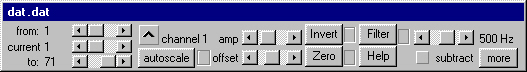
 This window comes in two variations, the more elaborate one is shown below (push the "less" control to see the window with less options). It is used to scale, to zero and to filter the input trace.
The toolbox
range from:
current:
range to:
12 Hz
![]() sweep range. The upper (marked "from:") and lower (marked "to:") slide bars are used to select either:
sweep range. The upper (marked "from:") and lower (marked "to:") slide bars are used to select either:
1) the range of records (sweeps) that will be used for analysis or
2) the range of records that will be displayed if in concatenated or family plot mode![]() .
.
The middle slide bar (marked "current") is to select the record currently displayed. If in concatenated or family plot mode![]() , the "current" record is highlighted.
, the "current" record is highlighted.
![]() channel. Push this button to show the next input channel (if any). Note that PClamp files that have been recorded using internally generated ramp stimulation show the ramp in the highest channel. |return|
channel. Push this button to show the next input channel (if any). Note that PClamp files that have been recorded using internally generated ramp stimulation show the ramp in the highest channel. |return|
![]() amplification. This slide bar changes the display amplification. It is only effective if autoscale is not set. Display amplification does not effect data analysis. |return|
amplification. This slide bar changes the display amplification. It is only effective if autoscale is not set. Display amplification does not effect data analysis. |return|
![]() autoscale. The data between the two vertical red lines in the input window are amplified to fit the window. Display amplification has no effect on analysis. |return|
autoscale. The data between the two vertical red lines in the input window are amplified to fit the window. Display amplification has no effect on analysis. |return|
![]() offset. Use this slide bar to add offset to the input data. This offset is also taken into account when data is analysed. To move the input trace up and down in the input window, use the vertical scroll bar at the right of the input window. To reset the offset to 0 (no offset), push the "zero" button twice. |return|
offset. Use this slide bar to add offset to the input data. This offset is also taken into account when data is analysed. To move the input trace up and down in the input window, use the vertical scroll bar at the right of the input window. To reset the offset to 0 (no offset), push the "zero" button twice. |return|
![]() zero. The average value between the vertical blue lines is subtracted from the entire sweep. This change in offset is also taken into account during analysis. Upon de-selection of auto-zeroing the offset is 0 (no offset). |return|
zero. The average value between the vertical blue lines is subtracted from the entire sweep. This change in offset is also taken into account during analysis. Upon de-selection of auto-zeroing the offset is 0 (no offset). |return|
![]() invert. Invert records. This also applies during analysis. |return|
invert. Invert records. This also applies during analysis. |return|
![]() filter. Low-pass filter on/off. The filter is a 2nd order phaseless recursive RC filter. |return|
filter. Low-pass filter on/off. The filter is a 2nd order phaseless recursive RC filter. |return|
![]() cut-off frequency. Select the low-pass 6dB cut-off point of the 2nd order filter with this slide bar. Filtering is taken into account during analysis. |return|
cut-off frequency. Select the low-pass 6dB cut-off point of the 2nd order filter with this slide bar. Filtering is taken into account during analysis. |return|
![]() 50 Hz removal. Removes 50 cycles and its first 6 harmonics. It is taken into account during analysis. |return|
50 Hz removal. Removes 50 cycles and its first 6 harmonics. It is taken into account during analysis. |return|
![]() 60 Hz removal. Removes 60 cycles and its first 6 harmonics. It is taken into account during analysis. |return|
60 Hz removal. Removes 60 cycles and its first 6 harmonics. It is taken into account during analysis. |return|
![]() activate subtraction. If subtraction sweeps have been selected or if leak compensation has been defined previously using the Conditioning>Subtraction set-up menu item, subtraction can be switched on or off. |return|
activate subtraction. If subtraction sweeps have been selected or if leak compensation has been defined previously using the Conditioning>Subtraction set-up menu item, subtraction can be switched on or off. |return|
![]() integration. If checked, the records are integrated. |return|
integration. If checked, the records are integrated. |return|
![]() differentiation. If checked, the records are differentiated. |return|
differentiation. If checked, the records are differentiated. |return|
If the "less" button is pushed, an alternative input tool window is displayed, containing less options. The 50&60 Hz removal, integration and differentiation options are absent and disabled in the "less options" tool window.
Basic data analysis using the cursors

1 2 3
Besides the arrow pointer, there are three cursors in the input window (marked 1,2 and 3 underneath the figure). Cursor 1 is used to move the vertical lines. The arrow pointer automatically changes into cursor 1 when it comes over a vertical line. These vertical lines or markers indicate the boundaries of the zero windowThe average value in between the vertical blue lines will be subtracted from the entire sweep. The blue lines are present only if the "zero" option in the input tool is active. The lines can be moved by dragging them with the mouse. (in blue) and the action window (in red).
The zero markers are used to indicate a stretch of each sweep that will be used as a reference or zero value (automatic zeroing): the average value of the data in between the blue markers is subtracted from the entire trace. The blue markers are visible only if the "zero" option in the input tool window is active, otherwise offset can be compensated using the "offset" slide bar.
The action window delineates the stretch of data in each trace that will be used for data analysis.
To move a marker, push the left mouse button when cursor 1 appears and drag the marker while keeping the mouse button depressed. Note that Zero windowsThe average value in between the vertical blue lines will be subtracted from the entire sweep. The blue lines are present only if the "zero" option in the input tool is active. The lines can be moved by dragging them with the mouse. and action windows are the same for each sweep but are independent for each input channel. Therefore, they need to be set separately for each input channel. However, to have identically positioned zero- or action-windows for all recorded channels, keep the <Ctrl> key depressed while moving the markers.
![]()
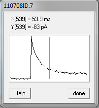
Cursors 2 (static) and 3 (dynamic) are used to manually measure x and y positions of the displayed data. When moving the mouse (arrow) pointer, cursor 3 follows it on the x-axis. If the right mouse button is clicked cursor 2 takes it place. If the mouse pointer is moved again, the status bar (see the figure above) displays the position of cursor 2, the current position of cursor 3 and the differences between them. The values between the square brackets indicate the index of the data point in the sweep (starting at index 0 at the beginning of the trace).
The keyboard can be used to move the two cursors:
* To move the cursor to the beginning of the trace: press the Home keyThe home key is a diagonally pointing arrow on the keyboard, located between the alphanumerical keypad and the numerical keypad in a group of 6 isolated keys..
* To move the cursor to the end of the trace: press the "end" key on the keyboard.
* To move the cursor a single data point (hence, NOT a single display pixel) to the left or the right press the left or right keys.
* To move the cursor faster to the left or to the right, depress the <Ctrl> key while depressing the arrow keys.
* To move the cursor to a local maximum within a range of 10 data points on the trace: press the up key. If the 'up' key is maintained depressed, the search continues. This facilitates searching a maximum value in the trace.
* To move the cursor to a local minimum, do similarly with the down key.
In order to move the static cursor 2 with the keyboard keys, depress the right mouse button while using the keyboard.
The values displayed in the status bar can be copied or transferred to a spreadsheet in several ways:
1) By pressing the "c" key. The data will be copied to the clipboard and can be pasted on a spreadsheet.
2) By pressing the "t" key. The data will be transferred immediately to the bottom line of a spreadsheet. If no spreadsheet is open, a new one will be created. If a single spreadsheet is open, the data will be pasted on that one. If more than one spreadsheet is open, a dialogue window will allow choosing between them or to create a new one. It is also possible to select a spreadsheet prior to transfer, or to change spreadsheet later, using the menu item Extract>Transfer manual input to....
3) By clicking the right mouse button. This action is the same as the "t" key.
The order of the data that appears in the spreadsheet columns is identical to that shown in the status bar. That is: first the position of the static cursor and then the position of the dynamic cursor (cursor 3). A few extra parameters appear in the last spreadsheet columns, such as the comment line and the values of the external variables (ep1 and ep2).
 Use the Magnifying glass command from the Window menu to enlarge the stretch of data centred around the currently active cursor (either one of the two red crosses). The magnifying glass helps to place the cursors correctly if the sweep contains many data points.
.
Plotmode
The Conditioning menu contains four plot mode entries, sweep plot modePer default, sweep plot mode
In family plot mode
Demo: "Graph directly from input" should be viewed full screen
Creating a graph directly from input data
1) The selected section of the current input sweep may be copied (by selecting the input window followed by pressing <Ctrl> C, by clicking the copy icon![]() in the icon bar or by selecting Edit>Copy as text from the menu of the input window). The contents of the clipboard may then be pasted onto a
drawing sheet or a spreadsheet by pressing <Ctrl> V, by clicking on the paste icon
in the icon bar or by selecting Edit>Copy as text from the menu of the input window). The contents of the clipboard may then be pasted onto a
drawing sheet or a spreadsheet by pressing <Ctrl> V, by clicking on the paste icon![]() in the icon bar or by selecting Edit>Paste from the menu of the drawing sheet or the spreadsheet.
in the icon bar or by selecting Edit>Paste from the menu of the drawing sheet or the spreadsheet.
If the contents of the clipboard are pasted on both the spreadsheet and the drawing sheet, the graph will be linked to the corresponding columns in the spreadsheet, meaning that a modification in one of the columns will alter the graph.
![]() Columns that maintain a link with a graph are marked by a '°' character in front of the column index.
A link can be removed by either clicking on the graph and selecting Edit>Remove Link from the drawing sheet menu or by selecting the columns and selecting Edit>Remove Links from the spreadsheet menu. The latter action will also remove links with other graphs that may exist on other drawing sheets. More on links
elsewhere.
Columns that maintain a link with a graph are marked by a '°' character in front of the column index.
A link can be removed by either clicking on the graph and selecting Edit>Remove Link from the drawing sheet menu or by selecting the columns and selecting Edit>Remove Links from the spreadsheet menu. The latter action will also remove links with other graphs that may exist on other drawing sheets. More on links
elsewhere.
2) A graph on a drawing sheet can be created in a single step using the input window's menu items Extract>Create XY line plot or Extract>Create bar plot (these menu items are not available if in concatenated plot mode![]() ). When selecting either of these menu items, a dialogue window
). When selecting either of these menu items, a dialogue window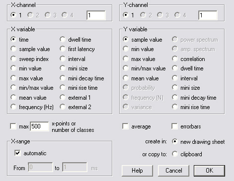 containing the following elements appears:
![]() X channel 1-16
X channel 1-16
Dat input files containing up to 16 channels that were recorded simultaneously can be read by the program. Select here which of the 16 provides the data for the x-coordinate. If less than four channels were recorded, the higher numbered check box![]() will be disabled. Use the edit box
will be disabled. Use the edit box![]() to enter an input channel number that exceeds 4.
to enter an input channel number that exceeds 4.
![]() Y channel 1-16
Y channel 1-16
Select here which of the 16 recorded input channels contains the data that will be used for the y-coordinate. The X and Y channels may be identical. Use the edit box![]() to enter an input channel number larger than 4.
to enter an input channel number larger than 4.
![]() y sample value
y sample value
Use this option if you wish to plot the recorded signal as a function of time. If the average option is not checked, the graph will display each selected sweep. If the average box is checked, the graph will contain a single trace representing the average of the selected traces.
![]() y min value
y min value
Sets the minimum value in the action windowThe section of a record that will be used for analysis is marked by the two vertical red lines. The red lines can be moved by dragging them with the mouse. of the sweep as the y-variable.
![]() y max value
y max value
Sets the maximum value in the action windowThe section of a record that will be used for analysis is marked by the two vertical red lines. The red lines can be moved by dragging them with the mouse. of the sweep as the y-variable.
![]() y min/max value
y min/max value
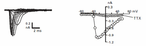
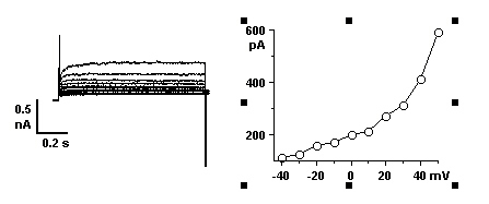
Sets either the minimum or the maximum value in the sweep as the y-variable, depending on which of the two has the largest absolute value. Use this option if you wish to plot the maximum value of each record. If used in conjunction with x-external 1 or 2, a current-voltage plot may be created:
![]() y mean value
y mean value
Sets the mean value in the action windowThe section of a record that will be used for analysis is marked by the two vertical red lines. The red lines can be moved by dragging them with the mouse. of the sweep as the y-variable. Use this option if you wish to plot the mean value of each record. If used in conjunction with x-external 1 or 2, a current-voltage plot may be created:
![]() y probability
y probability
Used in conjunction with x sample value, x dwell time, x-first latency, x interval, x mini size, x mini decay time or x mini rise time. Creates a histogram depicting a probability-density histogram or a dwell-time histogram. Dwell time histograms require either "idealised" data stored in a *.cha fileA *.cha file is a file in Electrophy-specific format, that contains (channel-) transition times and states. or synaptic events stored in a *.blb fileA *.blb (blib) file is a file in Electrophy-specific format, that contains the times of occurrence of synaptic currents/potentials. Data files can be idealised using either one of the menu items Conditioning>Idealise channels or Conditioning>window discrimination. Conditioning>Idealise channels may be used to detect channel openings or to re-digitise the data at a lower resolution and Conditioning>window discrimination may be used to detect spike events. For the detection of spontaneous synaptic currents/potentials click here.
![]() y frequency (N)
y frequency (N)
Identical to "probability", except that the surface under the curve is not normalised to unity.
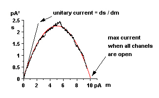
![]() y variance
y variance
Sets the variance as the y coordinate. Used in conjunction with x mean value. A so-called variance-to-mean histogram will be created. The histogram may then be fitted with a parabola from which single channel properties may be deduced (Neher & Stevens (1977) Annual Review of Biophysical Bioengineering 6, 345-381, see exercise 16 in Electrophyhelp.doc).
The relation between variance (s(p)) and mean (m(p)) is:
s(p) = i.m(p)-m(p)2/N,
with p the probability of channel opening that has to vary systematically in each sweep of an ensemble, i the unitary current and N the total number of channels. Differentiation of s with respect to m gives:
ds/dm=i -2.m/N.
Hence at zero mean current (p=0): ds/dm=i. fitting the histogram with a parabola:
s(x)=a+b.(x-x0)2 gives two equations:
at x=0: ds/dx = -2.b.x0 = i and at the intersection of the parabola with the y=s(x)=0 axis: x=N.i.
![]() y correlation
y correlation
Creates the autocorrelation histogram if the selected x and y channels are the same. If not, the cross correlation between the two channels is calculated. Used with x time.
![]() y power spectrum
y power spectrum
Used with x frequency. Creates the power spectrum of selected records.
![]() y amplitude spectrum
y amplitude spectrum
Used with x frequency. Creates the amplitude spectrum of selected records.
![]() y dwell time
y dwell time
If used in conjunction with x time, the evolution of the dwell time as a function of time will be shown. If used in conjunction with x sweep index, the evolution of the average dwell time per sweep will be shown. If used in conjunction with x external 1 or 2, the dwell time as a function of an external parameter will be plotted. This option is used only with "idealised" *.cha filesA *.cha file is a file in Electrophy-specific format, that contains (channel-) transition times and states.. Data files can be idealised using either one of the menu items Conditioning>Idealise channels or Conditioning>window discrimination. Conditioning>Idealise channels may be used to detect channel and Conditioning>window discrimination may be used to detect spike events.
![]() y interval
y interval
If used in conjunction with x time, the evolution of time intervals as a function of time will be shown. If used in conjunction with x sweep index, the evolution of the average interval per sweep will be shown. If used in conjunction with x external 1 or 2, the interval as a function of an external parameter will be plotted. This option is used only with idealised *.cha filesA *.cha file is a file in Electrophy-specific format, that contains (channel-) transition times and states..
![]() y mini size
y mini size
Plot the size of synaptic currents as a function of another feature of the minis. Before using this option, the minis need to be detected using a template.
![]() y mini decay time
y mini decay time
Plot the time constant of decay of synaptic currents as a function of another feature of the minis. Before using this option, the minis need to be detected using a template. Example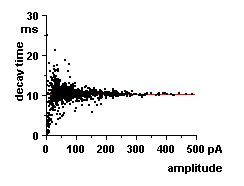 .
.
![]() y mini rise time
y mini rise time
Plot the rise time of synaptic currents (defined by the time interval between the 10% and 90% points relative to the peak (100%)) as a function of another feature of the minis. Before using this option, the minis need to be detected using a template.
![]() x time
x time
Sets time as the x-coordinate. Depending on the context, time=0 represents either the beginning of each sweep or the time of creation of the first sweep in a file. Hence, if choosing max value vs. time, time represents the intervals between creation of each sweep, while if choosing sample value vs. time, time represents the time lapse since the beginning of the sweep.
![]() x sample value
x sample value
Sets the sample value as the x-coordinate. This may be useful when plotting stimulus-response relations if both stimulus and response were recorded simultaneously on separate channels. Hence if a voltage-ramp was recorded on channel 2 and current on channel 1, plotting sample value (channel 1) vs. sample value (channel 2) gives an IV curve. Note that if a response to a ramp was recorded using Axoclamp software, the ramp is simulated in the highest channel upon loading of the file.
![]() x sweep index
x sweep index
Sets the record number as the x-coordinate. The first record (sweep) used for the analysis gets value 0. This option can be used only with y-variable selections that yield a single value such as y max value and y min/max value.
![]() x min value
x min value
Sets the minimum sample value in the action windowThe section of a record that will be used for analysis is marked by the two vertical red lines. The red lines can be moved by dragging them with the mouse. of the record as the x-coordinate.
![]() x max value
x max value
Sets the maximum sample value in the action windowThe section of a record that will be used for analysis is marked by the two vertical red lines. The red lines can be moved by dragging them with the mouse. of the record as the x-coordinate.
![]() x min/max value
x min/max value
Sets either the maximum or minimum sample value in the action windowThe section of a record that will be used for analysis is marked by the two vertical red lines. The red lines can be moved by dragging them with the mouse. of the record as the x-coordinate depending on which of the two has the largest absolute value.
![]() x mean value
x mean value
Sets the mean sample value in the action windowThe section of a record that will be used for analysis is marked by the two vertical red lines. The red lines can be moved by dragging them with the mouse. of the record as the x-coordinate if used in conjunction with y max or y min/max value. If used in conjunction with y variance however, a mean-to-variance plot is created. In this case the mean of the ensemble of records is taken at particular phase in the record. The number of means or xpoints calculated depends on the setting in the max xpoints edit box![]() .
.
![]() x frequency (Hz)
x frequency (Hz)
Sets frequency (Hz) as the x-coordinate. Use it to plot spectra.
![]() x dwell time
x dwell time
This option is used only with "idealised" *.cha filesA *.cha file is a file in Electrophy-specific format, that contains (channel-) transition times and states.. It is used to create dwell time histograms. Data files can be idealised using either one of the menu items Conditioning>Idealise channels or Conditioning>window discrimination. Conditioning>Idealise channels is used to detect channel openings and Conditioning>window discrimination may be used to detect spike events.
![]() x first latency
x first latency
This option is used only with idealised *.cha filesA *.cha file is a file in Electrophy-specific format, that contains (channel-) transition times and states.. It may used to create histograms that plot the probability that an event occurs after the onset of a stimulus as a function of time. See also x dwell time
![]() x interval
x interval
This option is used with either idealised *.cha filesA *.cha file is a file in Electrophy-specific format, that contains (channel-) transition times and states. or minis. It is used to create time interval histograms. In contrast to the dwell-time histogram it plots the interval between up- or down-going flanks of the "idealised" signal. See also x dwell time. Example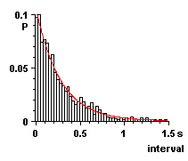 .
.
![]() x mini size
x mini size
A probability-density function of the sizes of spontaneous synaptic currents (minis) or a graph of some other feature of the minis (e.g. their decay times) as a function of mini size can be made using this option. Before using this option, the minis need to be detected using a template. UP↑
![]() x mini decay time
x mini decay time
A probability-density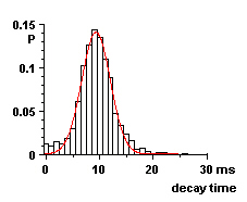 distribution of the single-exponential decay time constants of spontaneous synaptic currents (minis) or a graph of some other feature of the minis (e.g. their sizes) as a function of mini decay time can be made using this option. Before using this option, the minis need to be detected using a template.
![]() x mini rise time
x mini rise time
A probability-density function of the rise times of spontaneous synaptic currents (minis) or a graph of some other feature of the minis (e.g. their sizes) as a function of mini rise time (defined by the time interval between the 10% and 90% points relative to the peak) can be made using this option. Before using this option, the minis need to be detected using a template.
![]() x external 1
x external 1
Each record or sweep has external parameters associated with it. These parameters may be entered manually using the Edit>external variables menu item. They may also have been imported automatically from Axoclamp *.dat files. In this case these parameters may represent voltage- or time-increments that were used during acquisition. By selecting min/max value vs. external 1 or 2, a current-voltage curve may be created. Choose Record info from the Edit menu to show the current external variables.
![]() x external 2
x external 2
As for external 1.
![]() average
average
Creates a histogram that displays the average rather than individual data points. The average is calculated by grouping data with the same x-value. If the data do not allow calculation of the average, this option remains unchecked (e.g.: this will happen if selecting max of record vs. record number).
If selecting x time and y sample value, leaving "average" unchecked, the result will be a histogram that displays each input record as a separate curve. Checking "average" gives a single curve representing the average of the input records.
![]() error bars
error bars
Creates a histogram with vertical (y) error bars. This option turns on the average check box![]() .
If the data do not allow calculation of the average, this option remains unchecked.
.
If the data do not allow calculation of the average, this option remains unchecked.
![]() max
max ![]() xpoints or number of classes
xpoints or number of classes
If you wish to limit the number of x-coordinates and hence the number of data points in the graph, check the "max" box and enter the maximum number of xpoints in the edit box![]() . This option remains checked and the number of classes (xpoints) needs to be entered if the graph in question is a frequency histogram such as in probability vs. sample value.
. This option remains checked and the number of classes (xpoints) needs to be entered if the graph in question is a frequency histogram such as in probability vs. sample value.
X-range
If the graph to be created is a probability histogram (y is "probability"), then the range of values on the X-axis can be set. In combination with "max number of classes" one can thus fix the bin width in a probability-density function or a dwell-time histogram.
![]() automatic With this option set, the range of x-values is automatically determined. Uncheck this option to enter the minimum and maximum x values in the "from" and "to" edit boxes
automatic With this option set, the range of x-values is automatically determined. Uncheck this option to enter the minimum and maximum x values in the "from" and "to" edit boxes![]() . UP↑
. UP↑
Create histogram in a ![]() new drawing sheet or on the
new drawing sheet or on the ![]() clipboard (both as a vector graph and as spreadsheet columns). By default, the histogram will be created in a drawing window of its own.
Remember, to copy the new histogram to another drawing sheet, select the histogram by clicking once on it, then copy or delete it (<Ctrl> C or <Ctrl> X or the Copy or Delete command from the Edit menu) and paste it (<Ctrl> V or the Paste command from the Edit menu) onto the other drawing sheet. If the "copy to clipboard as" option is selected, the histogram and data columns will be created on the clipboard. Note: nothing seems to happen until the paste command is issued.
clipboard (both as a vector graph and as spreadsheet columns). By default, the histogram will be created in a drawing window of its own.
Remember, to copy the new histogram to another drawing sheet, select the histogram by clicking once on it, then copy or delete it (<Ctrl> C or <Ctrl> X or the Copy or Delete command from the Edit menu) and paste it (<Ctrl> V or the Paste command from the Edit menu) onto the other drawing sheet. If the "copy to clipboard as" option is selected, the histogram and data columns will be created on the clipboard. Note: nothing seems to happen until the paste command is issued.
Create PSTH
Classically, the PSTH displays the spike density following the onset of a repetitive stimulus (Post Stimulus Time Histogram) or the threshold-crossing of a periodical stimulus (Peri Stimulus Time Histogram). With Electrophy, the average spike interval or instantaneous frequency(1/interval) rather than the spike density may be displayed as well. To choose between these three possibilities, select 'density', 'interval' or instantaneous 'frequency' in the dialogue box that comes up. The PSTH will then show the spike number, the average spike interval or instantaneous frequency as a function of time elapsed after the left action windowThe section of a record that will be used for analysis is marked by the two vertical red lines. The red lines can be moved by dragging them with the mouse. marker (the left red vertical line in the input window). The average is taken over the number of sweeps as set in the action range. Before using this option, the spike events have to be detected using the window discrimination item from the Conditioning menu. After selecting Create PSTH from the menu the PSTH dialogue window pops up. Choose whether you wish to measure the intervals between up-going or down-going events, whether you wish error bars to be plotted and (optionally) what the number of x-points (classes or bins) should be. If the "max" box is left unchecked, the program will set the number of x-points to twice the average number of up- or down-going events per sweep. Error bars can only be plotted with the 'interval' and 'frequency' options and will not appear with 'density'.
Detection of single channel transitions
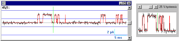
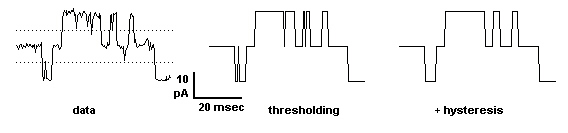
Before analysis of single-channel dwell times, the records containing the channel openings and superimposed noise need to be "idealised". This is a process that is very similar to analogue-to-digital conversion and consists of dividing the signal into a limited number of current steps. In this case, each step having exactly the size of the unitary current. To transform the input records into "idealised" unitary current steps, choose Conditioning>Idealise channels from the input window menu. A dialogue window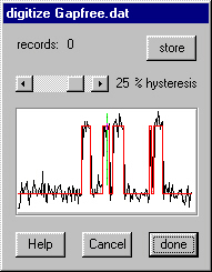 pops up and a series of blue horizontal lines appear in the input window. The blue lines indicate the thresholds between digitisation (current) levels. The result of the digitisation using the current threshold settings is displayed in red colour. If the mouse arrow pointer moves over one of the threshold lines it changes in to a
 ![]() pointer. Now, when depressing the left mouse button, the blue lines can be moved upwards or downwards. This changes the threshold settings and upon release of the mouse button, the result of digitisation is displayed as in the figures underneath:
pointer. Now, when depressing the left mouse button, the blue lines can be moved upwards or downwards. This changes the threshold settings and upon release of the mouse button, the result of digitisation is displayed as in the figures underneath:
The status bar shows the distance between levels: ![]() see also exercise 14 in the Electrophyhelp.doc file.
see also exercise 14 in the Electrophyhelp.doc file.
Somewhere in the middle of the input window a green vertical line has appeared. This green line indicates the centre of an area that is shown in greater detail in the dialogue window on a one pixel/data point basis (right figure). To move the green line, activate the input window if it is not yet active (by clicking on it), then click where you want the new centre to be or move the left or right arrows on the keyboard. Pressing one of the arrows, while holding the Before analysis of spike interval times, the records containing the spike activity need to be "idealised". Choose Conditioning>window discrimination from the input window menu. A dialogue window pops up and a two blue horizontal lines appear in the input window. These two blue line represent two thresholds. If the input signal traverses the lower blue line upwards once and downward once, without having passed the upper blue line, a "spike event" is detected and displayed by a red pulse-like signal. If the mouse arrow pointer moves over one of the threshold lines it changes in to a
Before the analysis of records containing randomly occurring synaptic currents (minis) can be carried out, the events need to be detected. The detection is done in two steps: Create a template
A template is used to facilitate the detection of synaptic currents or potentials in the data traces. When choosing Create mini template from the Conditioning menu, a dialogue window pops up that shows 6 options to create such a template. The "detection by template" dialogue window
After having defined a template, the occurrence of minis can be detected by issuing the Mini detection by template command from the Conditioning menu. If minis had not been detected in a previous session (no *.blb file found), Electrophy analyses the first 3 sweeps in the given range of sweeps using default parameters to estimate a threshold of detection. Then the "detection" dialogue window pops up and detection can begin. When using the File>Save command, the current input file will be saved in a Electrophy-specific format (*.dat), irrespective of the original file format.
With the File>Save as command, the data may be saved in Electrophy-specific format (*.dat) or it may be exported in tab-delimited ASCII (text). First, set the range of sweeps you wish to export using the "from" and "to" slide bars The third option, File>Save as wav, has no utility whatsoever, but it may be fun to hear your single-channel or spike recording using Windows media player. The range of sweeps of the currently selected channel is stored as a mono audio trace in wav format at a sample frequency of 11025 Hz.
Baseline correction
Per default the option
A node may be deleted by right mouse clicking on it.
The generation of new nodes is disabled after selection of move node. This is useful in windows particularly cluttered by nodes. Deletion of nodes is then still possible using the right mouse button.
Pushing the "clear all" button removes all nodes and unchecks the "enable" box.
Use the record slide bar Note that in "sweep plot mode Leak & sweep subtraction Multiply subtraction buffer Mini simulation
The Edit menu of the input window groups, as the name indicates, a certain number of edit functions. As nothing can be pasted to this window, a paste function is absent. In order to export the record shown in the window to other programs, such as bitmap-, vector- or text-oriented programs the data can be copied to the clipboard in one of the appropriate formats and then pasted in the receiving program. The Edit>Copy as text menu item is also available in the form of the copy icon Copy preferences. Calibration. External variables. Copy Externals. Record info. Save prefs. With the menu items Extract>Create XY line plot and Extract>Create bar plot a vector graph on a drawing sheet can be created directly starting from the input data. After selecting one of these menu items, a dialogue window will pop up asking to specify which will be the parameters of the data that will be used for x and y axes. For example, selecting x:'frequency' and y:'power' will result in the (average) power spectrum of the current range of sweeps. Create dot plot Create PSTH
Concatenated plot. Number of channels. Transfer manual input to ...
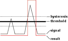
With the horizontal slide bar![]() in the dialogue window, a certain amount of hysteresis may be added to the thresholds (expressed as a percentage of the distance between two threshold levels).
in the dialogue window, a certain amount of hysteresis may be added to the thresholds (expressed as a percentage of the distance between two threshold levels).
 If a convenient result is thus achieved, press the "store" button in the dialogue window. The data are now stored in a temporary file and the next input record is displayed in the input window. Note that the "store" button now has a dotted rectangle around the button text. This means that if the
 ![]() s from the input tool window to select another input record. The "cancel" button is there to quit the session. When pushing the "done" button, a new dialogue window pops up requesting a file name to rename the temporary file. If you do not wish to keep the data choose "cancel". In that case, the temporary data file is still available for further analysis. However, it will be deleted upon closing its associated window. idealised data are stored in *.cha format. Note that, if in concatenated plot mode
s from the input tool window to select another input record. The "cancel" button is there to quit the session. When pushing the "done" button, a new dialogue window pops up requesting a file name to rename the temporary file. If you do not wish to keep the data choose "cancel". In that case, the temporary data file is still available for further analysis. However, it will be deleted upon closing its associated window. idealised data are stored in *.cha format. Note that, if in concatenated plot mode![]() , the plot mode returns to sweep mode temporarily. UP↑
, the plot mode returns to sweep mode temporarily. UP↑
Detection by window discrimination
![]() pointer. Now, when depressing the left mouse button, the blue line can be moved upwards or downwards. This changes the threshold setting and upon release of the mouse button, the new result of the window discrimination is displayed.
pointer. Now, when depressing the left mouse button, the blue line can be moved upwards or downwards. This changes the threshold setting and upon release of the mouse button, the new result of the window discrimination is displayed.
With the slide bar![]() , a certain amount of hysteresis may be added to the lower threshold (expressed as a percentage of the distance between the two threshold levels).
, a certain amount of hysteresis may be added to the lower threshold (expressed as a percentage of the distance between the two threshold levels).
After a convenient result is thus achieved, press the "store" button in the dialogue window. The data are now stored in a temporary file and the next input record is displayed in the input window. Note that the "store" button now has a dotted rectangle around the button text. This means that if the ![]() s from the input tool window to select another input record. The "cancel" button is there to quit the session. When pushing the "done" button, a new dialogue window pops up requesting a file name to rename the temporary file. If you do not wish to keep the data choose "cancel". In that case, the temporary data file is still available for further analysis. However, it will be deleted upon closing its associated window. Transition data is stored in *.cha format. Note that, if in concatenated plot mode
s from the input tool window to select another input record. The "cancel" button is there to quit the session. When pushing the "done" button, a new dialogue window pops up requesting a file name to rename the temporary file. If you do not wish to keep the data choose "cancel". In that case, the temporary data file is still available for further analysis. However, it will be deleted upon closing its associated window. Transition data is stored in *.cha format. Note that, if in concatenated plot mode![]() , the plot mode returns to sweep mode temporarily.
, the plot mode returns to sweep mode temporarily.
Detection of synaptic currents
Step 1 involves the creation of a template that resembles more or less the shape of the average mini. The shape of the template is not very critical, but it helps to prevent false detections and missing real ones. Usually, a prompt rise, 10 ms decay template works fine (the default).
Step 2 is the actual detection itself. An auxiliary file is created with the extension *.blb that contains the time of occurrence of each mini and the parameters, such as the template, that were used for the detection. This auxiliary file will be read-in the next time the *.dat file is re-opened. It is necessary that the *.blb file and the *.dat file reside in the same folder, so when moving the name.dat file, also move the name.blb file. After having detected the minis, graphs depicting size, interval and decay time histograms can be created using the Extract>Create XY Plot from the menu.
Options 1, 2 and 3 consist of a single exponential function with a prompt, linear and an exponential rising phase respectively. The time constants of rise and decay (in milliseconds) are entered in the edit boxes![]() at the right of these options. Any other function of the users design can be entered with the option "user-defined function". The latter function may only contain time (t) as a dependent variable and should be in seconds. If an error is encountered in the function definition, the dialogue window will refuse to close upon exit and an error message will be written underneath the function edit box
at the right of these options. Any other function of the users design can be entered with the option "user-defined function". The latter function may only contain time (t) as a dependent variable and should be in seconds. If an error is encountered in the function definition, the dialogue window will refuse to close upon exit and an error message will be written underneath the function edit box![]() . The set of functions allowed and syntax is the same as for the fitting functions. If the frequency of minis is relatively high and their sizes are large, a template can be automatically generated using option "square root of autocorrelation function". The idea behind this is that if the records are largely dominated by the synaptic currents and if background noise is negligible, the autocorrelation function will represent the "average" mini. However, if mini frequency is low, this method will yield garbage. The last option is "get from clipboard". This option may serve one of two goals:
. The set of functions allowed and syntax is the same as for the fitting functions. If the frequency of minis is relatively high and their sizes are large, a template can be automatically generated using option "square root of autocorrelation function". The idea behind this is that if the records are largely dominated by the synaptic currents and if background noise is negligible, the autocorrelation function will represent the "average" mini. However, if mini frequency is low, this method will yield garbage. The last option is "get from clipboard". This option may serve one of two goals:
1) It can be used to copy a template associated with one data file to another. To do so, activate the input window corresponding to the donor data file, select Conditioning>Copy template to clipboard.
2) The second goal is to use one or two columns of data in a spread sheet or a histogram in a drawing sheet, representing for example an average synaptic current, as a template. To do so, copy the column(s) or the histogram to the clipboard and select option "get from clipboard".
There are a few limitations to this method: the timebases (interval between data points) of the data in columns or histogram need to exactly match the timebase in the data file. If a single spreadsheet column is copied, the data file timebase is assumed. If two columns are copied, the first one needs to contain the time axis, and if it does not match the data file time base, an error message is issued. If a histogram is copied containing multiple curves, only the first in the list is considered.
After having created the template one might wish to visualise its shape. To see what it looks like, select Conditioning>Copy template to clipboard from the menu and paste the contents of the clipboard on a drawing sheet (by pressing <Ctrl>
V, by clicking on the paste icon![]() in the icon bar or by selecting Edit>Paste from the menu).
in the icon bar or by selecting Edit>Paste from the menu).
With method 1, synaptic currents are detected by deconvolution of the data by a template that the user has provided. If the number of synaptic currents per trace is low and the synaptic currents rise and decay slowly, then the deconvolved signal is very noisy and detection does not work well. There are two solutions: One could record the currents at a slower timebase, which increases the number of minis per trace and it shortens the synaptic current (in sample points), but one looses resolution.
The second solution is to use a slightly different method of detection: Rather than deconvolving, one can convolve data and template and search for maxima. As the convolved signal is very smooth, multiple stacked minis are almost never detected correctly. Because of this inconvenience the method is not recommended, but is included in case the first method fails. In the "detection" dialogue box the two methods are labelled "method 1" and "method 2" respectively. The use of the two methods may be mixed, that is, method 1 may be used for some sweeps and method 2 for others.
Use the vertical slide bar![]() to set the detection threshold as a function of (estimated) background noise. The dialogue window shows a somewhat pessimistic estimation of false positive detections per sweep at the current threshold setting. A threshold value resulting in approximately 1 false positive/sweep is a reasonable starting point (If the data are relatively free of noise a lower setting can be ventured). Then push the Do sweep button to see the result of the analysis of the current sweep. The input window and the dialogue window will show a result as in the figures underneath:
to set the detection threshold as a function of (estimated) background noise. The dialogue window shows a somewhat pessimistic estimation of false positive detections per sweep at the current threshold setting. A threshold value resulting in approximately 1 false positive/sweep is a reasonable starting point (If the data are relatively free of noise a lower setting can be ventured). Then push the Do sweep button to see the result of the analysis of the current sweep. The input window and the dialogue window will show a result as in the figures underneath:
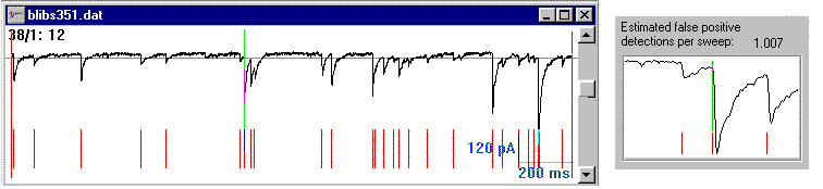 The left figure depicts the input window with spontaneous synaptic currents. The short red lines underneath show the instants where a match with the template has been found (pointing at the start of the template and NOT at another feature of the mini, such as its peak). Somewhere in the middle a green vertical line has appeared. This green line indicates the centre of an area that is shown in greater detail in the dialogue window on a one pixel/data point basis (right figure). To move the green line, activate the input window if it is not yet active (by clicking on it), then click where you want the new centre to be or move the left or right arrows on the keyboard. Pressing one of the arrows, while holding the
If there are missed events in the record, lower the threshold. If there are only few false detections, move the green line to the false event and press either the "d" (delete) key or <Ctrl>
X keys to remove the event. If the green line is not close enough to an event when the "d" key is depressed, Electrophy emits a beep. If the record contains large (stimulation) artefacts, move the large vertical red lines, such that this artefact lies outside their range and press the Do sweep button again. The next sweep to analyse can be indicated by moving the horizontal slide bar![]() in the dialogue window or by pressing the "n" (next) or "p" (previous) keys on the keyboard. Once the appropriate settings have been found, push the Do all button. To remove the results of a single sweep in the given range of sweeps, use the Clear sweep button.
in the dialogue window or by pressing the "n" (next) or "p" (previous) keys on the keyboard. Once the appropriate settings have been found, push the Do all button. To remove the results of a single sweep in the given range of sweeps, use the Clear sweep button.
The File menu
![]() in the input tool window. Then from the File>Save as dialogue box select the "ASCII" file format. After pushing the "OK" button, a dialogue window will pop up proposing two options:
If the "timebase in first column" option is set, the first column of ASCII data will contain the timebase (in ms) of the records that follow.
If the "units in first row" option is set, the first row will contain the units of the associated columns, i.e. "ms", "mV", "pA" or other build-in or user-defined units.
in the input tool window. Then from the File>Save as dialogue box select the "ASCII" file format. After pushing the "OK" button, a dialogue window will pop up proposing two options:
If the "timebase in first column" option is set, the first column of ASCII data will contain the timebase (in ms) of the records that follow.
If the "units in first row" option is set, the first row will contain the units of the associated columns, i.e. "ms", "mV", "pA" or other build-in or user-defined units.
According to your choice, the ASCII file will have the extension *.etf or *.txt and can be subsequently read by Electrophy, MSExcel or other programs that accept tab-delimited ASCII. Contrary to the *.txt format, the *.etf file contains additional non-ASCII information that appears after the "END OF FILE" string.
After the optional first column, the next columns will contain channel-1 of sweep-1, channel-2 of sweep-1 ...... channel-n of sweep1, followed by channel-1 of sweep-2, channel-2 of sweep-2 ..... channel-n of sweep-m, where n = the number of channels per sweep and m = the number of sweeps selected in the input tool window. Hence the file will contain n*m (+1) columns.
The Conditioning menu
Prior to data analysis, each sweep in a *.dat file or the file as a whole may be corrected for slow baseline fluctuations using the input window menu option Conditioning>Baseline correction. Upon selection of this menu item a dialogue window pops up and the input sweep is re-displayed with the input tool options "zero ", "invert" and "filter" disabled temporarily.
Select the "All records in range" check box![]() to correct the baseline for an ensemble of sweeps. Leave it unchecked to correct the baseline for each sweep separately.
to correct the baseline for an ensemble of sweeps. Leave it unchecked to correct the baseline for each sweep separately.
![]() add node is activated in the dialogue window. When clicking anywhere in the input window, a node, depicted by a red box, is added. As soon as more than one node is entered, a cubic spline passing through the nodes is displayed as a red line.
add node is activated in the dialogue window. When clicking anywhere in the input window, a node, depicted by a red box, is added. As soon as more than one node is entered, a cubic spline passing through the nodes is displayed as a red line.
If the ![]() enable box is checked, the spline is subtracted from the input data. In the latter case, nodes can still be added or moved, to fine-tune the result (it is a bit slower though, especially when in concatenated plot mode
enable box is checked, the spline is subtracted from the input data. In the latter case, nodes can still be added or moved, to fine-tune the result (it is a bit slower though, especially when in concatenated plot mode![]() ). If in the "add node" mode of operation, a new node is generated each time the left mouse button is clicked, except if clicked in the red box depicting a previously entered node. In that case, the position of the node may be changed by dragging it to a new location, while keeping the left mouse button depressed.
). If in the "add node" mode of operation, a new node is generated each time the left mouse button is clicked, except if clicked in the red box depicting a previously entered node. In that case, the position of the node may be changed by dragging it to a new location, while keeping the left mouse button depressed.
![]() to proceed to the next record in the file and the
to proceed to the next record in the file and the ![]() channel push button to move to the next input channel.
channel push button to move to the next input channel.
![]() ", spline subtraction must be enabled for each sweep separately and does not apply to the ensemble of sweeps. To turn baseline correction on or off, return to the Conditioning>Baseline correction dialogue window and check/uncheck the enable box.
", spline subtraction must be enabled for each sweep separately and does not apply to the ensemble of sweeps. To turn baseline correction on or off, return to the Conditioning>Baseline correction dialogue window and check/uncheck the enable box.
Either leak or a common signal may be subtracted from each input record by activating the subtract check box![]() in the input tool window. However, before subtracting anything, it should be defined what to subtract. Choose the Conditioning>Subtraction set-up menu item to set-up subtraction for the currently active input data file.
in the input tool window. However, before subtracting anything, it should be defined what to subtract. Choose the Conditioning>Subtraction set-up menu item to set-up subtraction for the currently active input data file.
1) Leak subtraction.
The "Subtract leak" option is available only if the input file contains information about the pulse protocol used and if the input window shows a current trace. Hence it works only for *.abf and clampex voltage-clamp records. Use the horizontal slide bar![]() to set the leak conductance and the "negative" checkbox to set its polarity. These leak compensation settings will then be applied to all records in the file, provided that the subtract checkbox in the input tool window is set.
to set the leak conductance and the "negative" checkbox to set its polarity. These leak compensation settings will then be applied to all records in the file, provided that the subtract checkbox in the input tool window is set.
The subtraction routine supposes that the leak reverses at 0 mV potential. If this is not the case, enter a value in the edit box![]() under the slide bar
under the slide bar![]() and push the '(reversal) potential offset' button.
and push the '(reversal) potential offset' button.
2) Common signal subtraction.
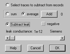 By choosing the "Select traces to subtract from records" option, a number of records in the file may be selected that will be used for subtraction. Either the sum or the average of the selected sweeps can be used, depending on the setting of the
 ![]() "sum" or
"sum" or ![]() "average" options. If the "add" button is pushed, the current sweep is added to the selection and the next record in the file is displayed. If the currently displayed record is not to be included in the selection, use the sweep range slide bar
"average" options. If the "add" button is pushed, the current sweep is added to the selection and the next record in the file is displayed. If the currently displayed record is not to be included in the selection, use the sweep range slide bar![]() s in the input tool window to move to a next record in the file. Use Conditioning>Multiply subtraction buffer to scale the subtraction buffer. The default is -1 (inversion).
In order to subtract a selection of sweeps from another document than the currently active document, make the selection of sweeps to subtract in the other document. Then activate the current document and select Conditioning>Subtraction borrow from the menu. A list of open input documents is displayed from which choice should be made. If this list window does not pop up, then none of the open input documents contains initialised subtraction data. The subtraction data from the selected document are then copied to the currently active document. If the number of data points/sweep in the donator document and the receiver document are different, the subtraction record is truncated or padded with zeroes as need be. Note that if the input window is in concatenated plot mode
s in the input tool window to move to a next record in the file. Use Conditioning>Multiply subtraction buffer to scale the subtraction buffer. The default is -1 (inversion).
In order to subtract a selection of sweeps from another document than the currently active document, make the selection of sweeps to subtract in the other document. Then activate the current document and select Conditioning>Subtraction borrow from the menu. A list of open input documents is displayed from which choice should be made. If this list window does not pop up, then none of the open input documents contains initialised subtraction data. The subtraction data from the selected document are then copied to the currently active document. If the number of data points/sweep in the donator document and the receiver document are different, the subtraction record is truncated or padded with zeroes as need be. Note that if the input window is in concatenated plot mode![]() , the plot mode returns to sweep mode temporarily.
, the plot mode returns to sweep mode temporarily.
Multiply the subtraction buffer by a scalar.
A *.dat file containing simulated minis will be generated when issuing the Conditioning>Mini simulation command from the input window menu. First a dialogue window pops up in which a certain number of parameters can be entered, such as the number of sweeps (each 4096 data points), the timebase (= time span of the sweep in seconds), the mini frequency in number of minis per second and the mini rise- and decay- time constants. The mini size can be kept constant or may be chosen Poisson distributed (an exponential probability distribution). Gauss distributed white noise can be added to the signal. The main purpose of this option is to let the user test the performance of the mini-analysis section of Electrophy and to get a feel about the limitations of the analysis. Clearly, estimation of mini amplitudes and kinetics will degrade with noise level. The figure below shows the estimated decay time (simulated time constant is 10 ms) as a function of mini size. Note that for smaller minis the estimates become less reliable.
Plot modes are described elsewhere.
The Edit menu
![]() in the icon bar. Use this menu item (or this icon
in the icon bar. Use this menu item (or this icon![]() ) to copy the data in between the two vertical red lines to a Electrophy or a Microsoft Excel spreadsheet (as two columns, one for the time axis (x) and one for the data (y)) or to a Electrophy drawing sheet (as a graph). The latter (i.e. "copy as text") may seem a bit odd, since Electrophy drawings are vector drawings and not text. This is done however, to create and maintain links between the spreadsheet text columns and graphs on a drawing sheet. Therefore, consider the text-copy icon as the general means to copy objects within Electrophy, whatever their format. Hence, Edit>copy as bitmap (in windows BMP format) and Edit>copy as vectors (in windows metafile, WMF, format) are for exportation only. If an input window trace is (icon- or text-) copied and then pasted both onto a spreadsheet and onto a drawing sheet, the two representations are linked, meaning that a modification of the data in the spreadsheet column will also change the graph. If copying when in "sweep plot mode
) to copy the data in between the two vertical red lines to a Electrophy or a Microsoft Excel spreadsheet (as two columns, one for the time axis (x) and one for the data (y)) or to a Electrophy drawing sheet (as a graph). The latter (i.e. "copy as text") may seem a bit odd, since Electrophy drawings are vector drawings and not text. This is done however, to create and maintain links between the spreadsheet text columns and graphs on a drawing sheet. Therefore, consider the text-copy icon as the general means to copy objects within Electrophy, whatever their format. Hence, Edit>copy as bitmap (in windows BMP format) and Edit>copy as vectors (in windows metafile, WMF, format) are for exportation only. If an input window trace is (icon- or text-) copied and then pasted both onto a spreadsheet and onto a drawing sheet, the two representations are linked, meaning that a modification of the data in the spreadsheet column will also change the graph. If copying when in "sweep plot mode![]() ", all data points in the record are copied to the clipboard, whereas only a maximum of 4096 points is copied when in "concatenated plot mode
", all data points in the record are copied to the clipboard, whereas only a maximum of 4096 points is copied when in "concatenated plot mode![]() ".
".
When exporting an input trace as vectors (WMF) to another program, the trace can be exported as a single polygon (single object) or as a series of line segments (multiple objects). Some programs find it difficult to dissociate a polygon into line segments, which makes it not easy to edit. Set your choice here.
Most often, the assignment of units (amperes, volts etc.) of the input data is carried out in the acquisition program and the user does not need to care about this. However, if you wish to change or to inspect the calibration, use this menu item. A dialogue window will pop up. It shows a number of fixed units on the left and a number of user-definable units next to them. If a new unit is entered, be sure that no more than 4 characters are used, it will be truncated otherwise. Fill in the conversion factor in the lower edit box![]() . Upon pushing the "apply" button, the new unit and/or conversion factor will be applied to the selected input channel and range of records in the file. (NB, Possibly, AxoGraph users may find the factor: "mV/unit" a bit occult. Do not worry, its just a scaling factor). Use the
. Upon pushing the "apply" button, the new unit and/or conversion factor will be applied to the selected input channel and range of records in the file. (NB, Possibly, AxoGraph users may find the factor: "mV/unit" a bit occult. Do not worry, its just a scaling factor). Use the ![]() to move to the next input channel and the slide bars
to move to the next input channel and the slide bars![]() to set the range of records. When closing the input window, Electrophy will ask whether or not to save the file. The file will be saved in a format, that can not be read by other software. Hence, it is best to use the File>save as menu option and to rename the file, such that the original data is still available for other programs. The following units are used by Electrophy: V, mV, µV, A, mA, µA, nA, pA, C, mC, µC, nC, pC, day, hr, min, s, ms, µs, KHz, Hz, mHz, nM, µM, mM, M. Hence, the program knows that 1 nA equals 1000 pA and that 1 A*s/V equals 1 C (Coulomb). Such conversions are not defined for user-defined units.
to set the range of records. When closing the input window, Electrophy will ask whether or not to save the file. The file will be saved in a format, that can not be read by other software. Hence, it is best to use the File>save as menu option and to rename the file, such that the original data is still available for other programs. The following units are used by Electrophy: V, mV, µV, A, mA, µA, nA, pA, C, mC, µC, nC, pC, day, hr, min, s, ms, µs, KHz, Hz, mHz, nM, µM, mM, M. Hence, the program knows that 1 nA equals 1000 pA and that 1 A*s/V equals 1 C (Coulomb). Such conversions are not defined for user-defined units.
Often the data in the input records are the result of a stimulation of some kind, such as electrical stimulation, drug application or light intensity. Two external variables can be entered for each input record. These external variables can be used to plot a response as a function of this variable. The edit box![]() es marked v1 and v2 take floating point numbers, while the edit box
es marked v1 and v2 take floating point numbers, while the edit box![]() es unit1 and unit2 take a character string (for example mA or nM). Usually the units do not change within a file. To prevent retyping the same string 300 times over, do the following: 1) move the slide bar upwards so as to edit the first edit box
es unit1 and unit2 take a character string (for example mA or nM). Usually the units do not change within a file. To prevent retyping the same string 300 times over, do the following: 1) move the slide bar upwards so as to edit the first edit box![]() in a column. 2) type the string. 3) push the "copy" button. 4) push the "replace" button. Note that the "replace" button is now the default button as indicated by a dotted rectangle around the button text. This means that on hitting the
in a column. 2) type the string. 3) push the "copy" button. 4) push the "replace" button. Note that the "replace" button is now the default button as indicated by a dotted rectangle around the button text. This means that on hitting the
AxoClamp stimulation parameters will be automatically entered in these columns.
A value can be added to all entries in the v1 or v2 column by pushing either the 'add to v1' or the 'add to v2' button. This may be useful to add for example the value of the holding potential to a series of relative impulse potentials. The values in the v1 and v2 columns can be multiplied in a similar fashion by pushing one of the 'multiply' buttons.
Under the "comment" column, a string of characters can be entered for information. This comment line will appear in the upper left corner of the input window.
This option copies the external variables to the clipboard for use in a spreadsheet.
This menu item creates a sort of browser showing physical units, external variables and comment lines. The data in the window can not be edited. Selecting a line in the window causes the corresponding input record to be read and displayed in the input window. Inversely, selecting a record using the input tool range slide bar![]() s, will highlight the corresponding entry in the input list window.
s, will highlight the corresponding entry in the input list window.
The input tool window takes certain default settings each time a new data file is opened. To define the settings corresponding to the currently active input window as the default, select this menu option. The current size of the input window will be the default size when a new file is opened. However, the settings in the notch, integrate and differentiate checkboxes will remain 'unchecked' per default.
The Extract menu
The Create>bar plot option is intended to make a bar diagram with equidistant bars, e.g. to compare means and standard error of two sets of data. Therefore when the actual bar plot is made on the drawing sheet, possibly not equidistant x-values are ignored and the y-values are plotted equidistantly anyway. Bar plots are more useful in connection with spreadsheet data than with raw input data. To give a bar-like appearance to a graph generated by Create XY line plot, double-click on one of the elements of the curve and choose ![]() bars from the "Curve properties" dialogue window. This bar-like appearance is the default when choosing for example the combination x:sample value and y:probability.
bars from the "Curve properties" dialogue window. This bar-like appearance is the default when choosing for example the combination x:sample value and y:probability.
This menu item allows a visual impression of the grouping of spikes at a certain phase of the input records. First the spike events have to be detected using the window discrimination item from the Conditioning menu. The dot plot plots each occurrence of an up-going (or down-going) event as a dot in a graph as a function of time (horizontal) and sweep number (vertical). As an example suppose that several traces were recorded containing spike activity in response to a stimulus synchronised to the data acquisition. If the preparation responded by an increase in spike frequency after say 100ms, then the density of dots will be higher at 100ms than elsewhere in the plot. For more details "Creating a graph directly from input data".
Classically, the PSTH displays the spike density following the onset of a repetitive stimulus (Post Stimulus Time Histogram) or the threshold-crossing of a periodical stimulus (Peri Stimulus Time Histogram). With Electrophy, the average spike interval or instantaneous frequency(1/interval) rather than the spike density may be displayed as well. To choose between these three possibilities, select 'density', 'interval' or instantaneous 'frequency' in the dialogue box that comes up. The PSTH will then show the spike number, the average spike interval or instantaneous frequency as a function of time elapsed after the left action windowThe section of a record that will be used for analysis is marked by the two vertical red lines. The red lines can be moved by dragging them with the mouse. marker. The average is taken over the number of sweeps as set in the action range. Before using this option, the spike events have to be detected using the Window discrimination item from the Conditioning menu. After selecting Create PSTH from the menu the PSTH dialogue window pops up. Choose whether you wish to measure the intervals between up-going or down-going events, whether you wish error bars to be plotted and (optionally) what the number of x-points (classes or bins) should be. If the "max" box is left unchecked, the program will set the number of x-points to twice the average number of up- or down-going events per sweep. Error bars can only be plotted with the 'interval' and 'frequency' options and will not appear with 'density'.
This menu option generates a graph in which the input records in the selected range are plotted sequentially. It can be used, for example, to plot a number of data blocks recorded with Axolab Fetchex. As the number of data points in the selected range of sweeps can be very large (eating memory and processor time), a dialogue window pops up requesting whether the number of points might be limited by either under-sampling (skipping data points) or averaging of adjacent data points. The edit box![]() in the dialogue box shows the actual number of data points unless it is larger than 32000.
Note that, as with almost all actions on input records, only data points between the red vertical lines in the input window are used for the concatenated graph. To use the whole trace, move the red lines to the beginning and the end of the input window. Note that this menu item gives similar (although not identical) results as copy/paste when in concatenated plot mode
in the dialogue box shows the actual number of data points unless it is larger than 32000.
Note that, as with almost all actions on input records, only data points between the red vertical lines in the input window are used for the concatenated graph. To use the whole trace, move the red lines to the beginning and the end of the input window. Note that this menu item gives similar (although not identical) results as copy/paste when in concatenated plot mode![]() .
.
This option applies only to *.cha filesA *.cha file is a file in Electrophy-specific format, that contains (channel-) transition times and states. (containing idealised channel transitions). The number of channels in the patch is estimated in two ways.
1) The simplest way is to find the maximum number of levels encountered in the range of records. This may be an over-estimation if artefacts (e.g. capacitive currents) are present. It may be an under-estimation if the probability of channel opening is low.
2) A more elaborate way is to apply a binomial analysis. If channels are all identical and independent of one another, then the probability-density function should obey the binomial distribution law. There are two unknowns, the probability of opening and the number of channels. By varying the hypothetical number of channels systematically and calculating the probability of opening of an individual channel, the program finds the best fit to the experimental density function. The approach is different if channel activity is at equilibrium or if it is evoked. In the latter case, it is assumed that the evolution of the probability of opening as a function of time is identical in each of the records in the range. It is up to the user to decide which of the conditions apply to his case.
When measuring signal amplitudes, delay times etc. in the input window manually, the cursor positions may be copied/transferred to a spreadsheet. This menu option defines to which spreadsheet this data will be transferred. If there are multiple open spreadsheets, a dialogue window will pop up requesting which of the available spreadsheets is to receive the data. Click on the spreadsheet of your choice and press the "OK" button.
Create white noise.
Creates a *.wav file containing white noise. In the dialogue window that pops up, select the sample frequency, number of channels (mono or stereo) and the duration of the record. After creation of the file, a new sound window opens showing the result.
Search the manual: