The main window
 The main window at startup is empty, but may contain multiple windows corresponding to as many documents later on. Some of the items of the drop down menu are represented as icons in the icon bar for rapid access. The two rightmost icons are to get (contextual) help. The status bar will give you often a hint of what an icon is for when hovering over it with the mouse pointer. In case of the drawing sheet, it shows the x and y coordinates of the mouse pointer in cm. When drawing a figure or a line it shows the object's dimensions.
The File menu
New
Choose here whether to create a new window to manipulate numerical data (spreadsheet) or a new window for vector drawing (drawing sheet)
.
Open
Opens an existing file in one of the allowed formats: his, etf, txt, csv, bmp, tif, jpg
Save, Save as and Save with links
The File menu contains three items that deal with saving your data on hard-disk: Save, Save As and Save with links. The Save As menu item prompts for a file name. It is not necessary to type the file extension (e.g. ".txt") in the "Save" dialogue box. The Save menu item, whose action is identical to the ![]() button in the icon bar, rewrites a file on disk after it has been modified by the user. It does not prompt for a file name. The Save command behaves as the Save As command if the document is a newly created one.
button in the icon bar, rewrites a file on disk after it has been modified by the user. It does not prompt for a file name. The Save command behaves as the Save As command if the document is a newly created one.
spreadsheets are saved with the extension ".txt" or ".etf". The first contains only simple text and can therefore be read by most word-processing programs. The latter contains additional non-ASCII information that appears after the "END OF FILE" string. Before writing the file on disk, cell references and function names are translated into a format that can be understood by the english version of MS Excel. However, not all functions that are provided by Serf have an equivalent in MS Excel (e.g. fdens(), sbar() and cdate) and will generate an error message. At this date, MS Excel does not (yet) support multiple languages, and hence a french version of Excel may not understand the function names in ".txt" files.
drawing sheets are saved with the extension ".his". They contain data in a format that is specific for Serf and thereby can not be read by other programs. To copy vector drawings to other programs use the Copy item in the Edit menu and paste the contents of the clipboard, which are then in Windows Matafile (WMF) format, in the receiving program. The WMF standard comprises a large number of functions and possibilities. In fact too large, since most programs, including Serf, do not care to handle all those functions and possibilities with the result that some aspects of the original drawing are lost in the receiving program. Recent versions of the programs of Microsoft, who is the inventor of WMF, are an exeption (e.g. Powerpoint): they display a drawing copied from Serf correctly.
Upon saving a drawing sheet with the Save command, the links between histograms and spreadsheets are lost. Generally this is not a problem, since the histograms contain all the data necessary to re-establish a new link with a new spreadsheet in case the need is felt to edit the histogram or to add new data points to it. Just copy the histogram to the spreadsheet. However, if most of the essential data are on the spreadsheet rather than on the drawing sheet, recreation of the graphs from the spreadsheet every time one reloads the spreadsheet may be somewhat tedious. This situation presents itself for example if the spreadsheet contains a number of slide bars![]() used to animate a graphical demonstration of a function. To save the drawing sheet and it's associated spreadsheets in a single file use the menu item Save with links. This file remains a ".his" file. Upon loading of a "linked" his file, the spreadsheets that were saved with it will be displayed and the links with the drawing sheet will be re-establised. The program remembers if the loaded drawing sheet was originally a "linked" file. This means that upon closing the window after an editing session, issuing the Save command or pushing the "save" button, the file will be saved per default with the linked spreadsheets.
used to animate a graphical demonstration of a function. To save the drawing sheet and it's associated spreadsheets in a single file use the menu item Save with links. This file remains a ".his" file. Upon loading of a "linked" his file, the spreadsheets that were saved with it will be displayed and the links with the drawing sheet will be re-establised. The program remembers if the loaded drawing sheet was originally a "linked" file. This means that upon closing the window after an editing session, issuing the Save command or pushing the "save" button, the file will be saved per default with the linked spreadsheets.
The drawing sheet may be saved as a Windows bitmap (*.bmp) or a Windows metafile (*.wmf). To do so, select the "bitmap" or "windows metafile" format from the "File>Save as" dialogue box. In the second dialogue box that will pop up, either the bitmap resolution or the WMF format version may be set. Enhanced WMF is required for some recent programs, but is not correctly treated by older ones.
Bitmaps are saved in windows *bmp format. To save a bitmap on a drawing sheet, first select a single bitmap and then 1) issue the save bitmap command from the bitmap menu or 2) click the ![]() button or 3) press <Ctrl>S. While action 1 prompts for the number of bitmap colours, actions 2 and 3 assume the last used colour depth. Hence, 2 and 3 are shortcuts. Note that if no bitmap is selected, <Ctrl>S will save the drawing sheet.
button or 3) press <Ctrl>S. While action 1 prompts for the number of bitmap colours, actions 2 and 3 assume the last used colour depth. Hence, 2 and 3 are shortcuts. Note that if no bitmap is selected, <Ctrl>S will save the drawing sheet.
Text file format.
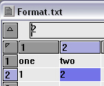
The program reads Tab delimited text files. The tabulation indicates a change of column. For example, the data on the spreadsheet below are coded as follows (with the ASCII code 9 designating the tabulation character and the ASCII code 13 designating a "carriage return" : o' 'n' 'e' 9 't' 'w' 'o' '10 '1' 9 '2' 13. Other file types exist that do not use a carriage return (13), but a line feed (10) and still others that use a comma instead of a TAB. Since a comma is used in many countries as a decimal sepatator, there can be confusion. A dialogue appears if the program is not sure of the file format.
Run a copy of the program
Per default, only one copy of the program is active. Use this option if you whish a second or third copy of XLPlot to run simultaneously.
Close
This menu item closes the currently active child window.
Printer setup
Choose your printer and its preferences. Use this menu iitem to change the page size (e.g. A4 or US-letter) and, in case of a drawing sheet, the orientation of the sheet (portrait or landscape).
Print
Print the contents of the currently active child window.
About
The "About" dialogue box provides information about the program version and whether an update is available. It also shows the file versions that are being written when selecting Save from the menu. The files are normally downward compatible but generally not upward compatible. Clicking the "Serf Software Suite" icon brings you to the program site. Reporting a problem will be anonymous unless you include a reply email address to discuss the problem.
Download update
Download the latest version of the program. This menu item is greyed out if your version is up to date or if the internet is not accessible.
How to deal with links between spreadsheets and drawing sheets
Establishing and removing links.
Links between a spreadsheet column and a graph are established in three ways.
1) By pasting the contents of the clipboard on both the spreadsheet and the drawing sheet.
2) By copying one or more spreadsheet columns and issuing the Modify/Stats>Line plot, Modify/Stats>Bar plot or the Modify/Stats>Wind rose plot from the spreadsheet menu.
3) By copying a graph and pasting it on a spreadsheet.
If a spreadsheet column and a graph on a drawing sheet are linked, data in the graph can be modified by modifying the numbers in the spreadsheet column. For example, removal of a spreadsheet cell will result in the removal of a data point in the graph. The modifications take effect immediately. There is an important exception to this rule: If an entire "linked" column is deleted from the spreadsheet, the plot on the drawing sheet will remain intact. The link is simply removed.
![]() Columns in a spreadsheet that maintain a link with a graph are marked by a 'º' character in front of the column index.
Columns in a spreadsheet that maintain a link with a graph are marked by a 'º' character in front of the column index.
A link can be removed by either clicking on the graph and selecting Edit>Remove Link from the drawing sheet menu or by selecting the columns and selecting Edit>Remove Links from the spreadsheet menu. The latter action will also remove links with other graphs on other drawing sheets if they exist. Hence, to remove only the link with one graph, select the graph and then choose the Edit>Remove Link item from the drawing sheet menu.
How to know what is linked to what?
To know whether a curve in a graph is linked to a spreadsheet and if so, to which column(s), double-click on an element (line segment or symbol) of the curve. The "curve properties" dialogue window appears. In the lower left corner of this window you find the name of the spreadsheet (if any) to which the curve is linked along with information about columns that contain the x, y and error bar data. Push the "next curve" button to find out to what columns the next curve in the graph is linked. In some cases, especially in very crowded graphs, a curve may be completely hidden by other curves that are drawn over it. In that case, select the column in the spreadsheet that is suspected to contain the data while depressing the control key on the keyboard.
![]() Now a question mark appears in the column index key. Then return to the graph and double click on any curve while depressing the control key. The "curve properties" dialogue window appears with information about which curve is linked to the spreadsheet column with the question mark.
Now a question mark appears in the column index key. Then return to the graph and double click on any curve while depressing the control key. The "curve properties" dialogue window appears with information about which curve is linked to the spreadsheet column with the question mark.
Demo: "Fit a parabola" is better viewed full screen
Fitting a function to data
Functions can be fitted to your data in each of the three types of window. The function can be one of the build-in functions (marked by an asterisk in the Fit dialogue window) or one that is defined by the user. Before starting the fit routine the user has to select or define i) the function to fit and ii) the range of data points to fit the function to. The way to do this differs slightly for each of the sheets.
The spreadsheet.
i) The fit routine requires two arrays of data: one for the x-values and one for the y-values. These data correspond to two columns that needs to be indicated. There are several ways to do this. a) By selecting a column and choosing Modify/Stats->Set X-column from the menu, then selecting a second column and choosing Modify/Stats->Set Y-column from the menu. An x and a y will appear in the column bar. A third column may be chosen using Modify/Stats->Set Error-column, that may be used as a weight during fitting. A second (more rapid) way is b) to select two columns (not less, not more), the first column will be considered to contain the x-data and the second will be considered to contain the y-data. If you wish c) to fit only a part of the numerical data in two adjacent columns, you may select the spreadsheet cells that contain the data to be fitted.
ii) Click the set fit function item from the Math menu to choose a function. To start the fit routine select Do fit from the same menu or click the fit icon.
The drawing sheet.
Only data in an undissociated graph can be fitted. Once a graph is dissociated, it is reduced to a simple set of vector elements. To fit one of the curves in a graph, double click on one of its elements (the line elements or the symbols, but not one of the axes of the graph) and a dialogue window will pop up containing, amongst others, two slide bar![]() s titled "fit range from" and "to" and three buttons saying "polynomial", "function" and "Do fit". Furthermore, two red vertical lines will appear in the graph.
s titled "fit range from" and "to" and three buttons saying "polynomial", "function" and "Do fit". Furthermore, two red vertical lines will appear in the graph.
i) Use the slide bars![]() to indicate which data points to fit.
to indicate which data points to fit.
ii) use the "function" button to select the fitting function. Then proceed by clicking "Do fit". To fit a polynomial push the "polynomial" button. A dialogue box comes up. Fill in the degree of the polynomial to fit, then check or uncheck which coefficients to fit or not. Use the buttons "even" and "odd" to fit only the coefficients of even and odd powers respectively.
The "Select Fit function" and "Fit" dialogue window.
To choose a function in this window, either double click one of the functions listed under "list of functions" or click once and push the "<<" button. The function name and its formula now appear in the upper left edit box![]() . The formula can be modified in order to create a new one. During compilation of a formula, lower case letters will be converted to upper case, hence the compiler does not distinguish between them. Before using the newly created formula, click the ">>" button to save it.
. The formula can be modified in order to create a new one. During compilation of a formula, lower case letters will be converted to upper case, hence the compiler does not distinguish between them. Before using the newly created formula, click the ">>" button to save it.
The variables to fit are listed underneath the edit box![]() . Do not attempt to use "X", "Y" or function names such as "exp" as variable names since they are reserved and will lead to unexpected results. The user can put constraints on the range of values that the fit parameters may adopt by checking V < 0 (variable must be negative), fixed (do not fit this parameter, but keep it constant) or V>0 (variable must be positive). The maximum of fit iterations can be set in the "iterations" edit box. The following functions may be used in fit formulas:
. Do not attempt to use "X", "Y" or function names such as "exp" as variable names since they are reserved and will lead to unexpected results. The user can put constraints on the range of values that the fit parameters may adopt by checking V < 0 (variable must be negative), fixed (do not fit this parameter, but keep it constant) or V>0 (variable must be positive). The maximum of fit iterations can be set in the "iterations" edit box. The following functions may be used in fit formulas:
Click the "cancel" or "OK" button to quit the fit dialogue window.
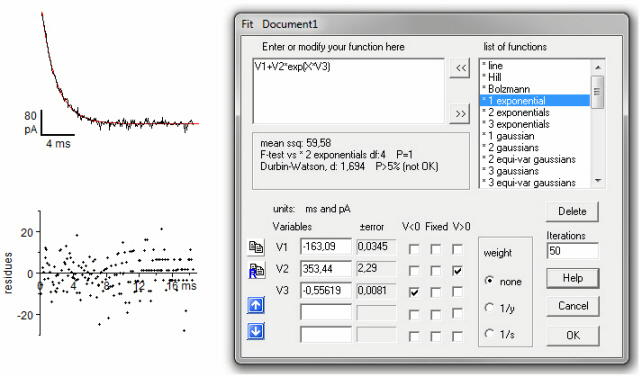
Start fitting by selecting "Do Fit" from the context described above. After estimation of the fit parameters, the same fit dialogue window pops up, now showing the estimated variables, the estimated error of each variable and the chi-2 error of fit underneath the formula edit box![]() . The program carries out the Fisher's F-test if a different function or the same function with different number of degrees of freedom has been fitted to the same data previously. The result of this test indicates whether the current function fits the data significantly better than the previous function. A P<0.05 indicates a significant difference.
. The program carries out the Fisher's F-test if a different function or the same function with different number of degrees of freedom has been fitted to the same data previously. The result of this test indicates whether the current function fits the data significantly better than the previous function. A P<0.05 indicates a significant difference.
In case of fitting a curve in an input window or drawing sheet the fitted function is drawn. The estimated parameters may be copied as text to the clipboard by pressing the copy icon: ![]() . in the fit dialogue window. The fit residues may be copied to the clipboard by pressing
. in the fit dialogue window. The fit residues may be copied to the clipboard by pressing ![]() . The clipboard contents can then be pasted onto a spreadsheet or a drawing sheet. The fit residues indicate whether you've chosen the a resonable function. If the function represents the correct model for the data, then the residues (differences between data and the fitted function (red in the figure below) will be randomly distributed above and below the zero line. The Durbin-Watson method tests this statistically. A probability larger than 5% signals a problem. In the figure below the Durbin-Watson tests suggests to try another function. Even so, fitting with two exponentials gave no better results, since the Fisher test gave no difference (P=1) between the two models. In such a case the function with the least number of parameters should be preferred (Ockam's rasor?).
. The clipboard contents can then be pasted onto a spreadsheet or a drawing sheet. The fit residues indicate whether you've chosen the a resonable function. If the function represents the correct model for the data, then the residues (differences between data and the fitted function (red in the figure below) will be randomly distributed above and below the zero line. The Durbin-Watson method tests this statistically. A probability larger than 5% signals a problem. In the figure below the Durbin-Watson tests suggests to try another function. Even so, fitting with two exponentials gave no better results, since the Fisher test gave no difference (P=1) between the two models. In such a case the function with the least number of parameters should be preferred (Ockam's rasor?).
Build-in fit functions are: line, Hill, Bolzmann, 1, 2 or 3 exponentials, Gaussians (1, 2 or 3, equidistant or both equidistant and equivariance), hyperbola, parabola, power, Lorentzians, logistic, log, log normal, Langmuir and sigmoids.
Linear regression.
If the first function (*line) of the list of functions is selected, a single step, linear regression routine is used rather than the iterative non-linear curve fitting routine. In that case, the correlation coefficient, r, and the probability, P, that correlation is absent between X and Y data is shown upon return.
The curve properties window contains a checkbox "confidence limits". If this box is checked, lines appear above and below the fitted function depicting the 95% confidence band. This means that there is a 95% probability that the mean Y value for a given X resides within this band.
Key commands
Common to all windows:
drawing sheet:
Spread sheet:
The formula Assistant
The formula assistant helps to create an equation in a spreadsheet cell. The first character in a formula has to be the "equal" sign, =, otherwise it will be considered as simple text. Select an operand (e.g. + ) or a function (e.g. sqrt ) from the list box and push "insert" to enter the function in the edit box![]() at the bottom of the assistant's dialogue box. A short description of the operand or function is given in the middle panel. Add brackets and function parameters as indicated in the latter panel. If you wish to insert a reference to a spreadsheet cell rather than a constant, click on the spreadsheet cell concerned. In order to change a spreadsheet cell reference that you entered previously, position the edit box cursor anywhere between the brackets delineating the reference and click on the new spreadsheet cell. To change the range of spreadsheet cells, proceed similarly.
Use the "verify" button to check for errors. If an error occurs, a new dialogue box will pop up displaying the probable cause of the error. Push the "help" button in this box to get more information. When done, push "OK".
at the bottom of the assistant's dialogue box. A short description of the operand or function is given in the middle panel. Add brackets and function parameters as indicated in the latter panel. If you wish to insert a reference to a spreadsheet cell rather than a constant, click on the spreadsheet cell concerned. In order to change a spreadsheet cell reference that you entered previously, position the edit box cursor anywhere between the brackets delineating the reference and click on the new spreadsheet cell. To change the range of spreadsheet cells, proceed similarly.
Use the "verify" button to check for errors. If an error occurs, a new dialogue box will pop up displaying the probable cause of the error. Push the "help" button in this box to get more information. When done, push "OK".