The drawing sheet

The Bitmap menu

The dialogue box shows the darkest or lowest intensity encountered in the bitmap as well as the brightest or highest intensity found. These numbers can be edited, or the red cursors can be moved to change the settings. Bitmaps can be exported similarly or by issuing the command Bitmap>Save bitmap or by pushing the button.

Save bitmap
This menu option is enabled if a single bitmap object is selected. Select the bitmap format in the first dialogue window that pops up. Note that the 16-bit bitmap (32768 colours, a Windows 3.x format) is now almost obsolete and most bitmap programs such as Photoshop and Corel Photopaint will refuse to load it.

Enter a file name in the next dialogue window that pops up. Note the difference with the menu item "Copy window as bitmap". Bitmaps can also be saved by clicking the button or by pressing <Ctrl> S. Select the number of bitmap colours and the file format (bmp,jpg or gif). Note that if no bitmap is selected, <Ctrl> S will save the drawing sheet (in *.his format).  

Size maps
With this option multiple bitmaps can be sized simultaneously. To do so, select the bitmaps to size and then issue the Size maps command from the Bitmap menu (or press <Ctrl>T). A dialogue box will pop up that allows you to choose between full size (1), one eighth, a quarter of or half the original size. Note that bitmaps may also be sized as any other object, i.e. : Select the object. It has 8 little squares around it. If the mouse cursor gets over one of them it changes into a vertically, horizontally or a diagonally pointing pair of arrows. Depress the right mouse button and drag the pointer until the object has the appropriate size. Use the corner squares to change dimension in two directions and use the other squares to change size in one direction only. In order to maintain the original proportions of the object (x and y amplification identical), press the <Ctrl> key and release it after having released the mouse button. A third way to size a bitmap is to double click on the image. In the dialogue box that appears, change the horizontal and vertical resolutions to the values of your choice.

Full screen
Use this option to display the currently selected bitmap full screen or type <Ctrl> O. Type the <escape> key to return to the program. If you have two display monitors, you may display a bitmap on the auxiliary monitor using <Ctrl> I.

Scale brightness
The colour of each pixel of a bitmap in this software is encoded by three bytes (a byte is a small integer number that can take on values between 0 and 255): one byte for the blue component, one for green and one for red. If the pixels in the bitmap have values that are all below 150 for example, then using Bitmap>Scale brightness>all multiplies all pixel values with a factor (255/150 in this case) such that the whole range of values between 0 and 255 is used. With using Bitmap>Scale brightness>Red only the red component is scaled. Scale brightness>Green and Scale brightness>Blue function similarly. Note that carrying out one after the other Scale brightness>Red, Scale brightness>Green and Scale brightness>Blue does not give the same result as Scale brightness>all, because in the latter case the scaling factor for all three components is the same and depends on the highest byte value found, irrespective of colour.

Adjust contrast
This menu option described in detail elsewhere.

Smooth
This menu option is enabled only if a single bitmap object is selected. The bitmap is passed through a 3x3-pixel (GaussianA Gaussian filter takes the weighed mean (a bell-shaped function) of the central pixel and its neighbour pixels. The mean is then attributed to the central pixel.) smoothing filter.
   Original + noise                  Smoothing filter                     Median filter

Remove noise
This menu option is enabled only if a single bitmap object is selected. The bitmap is passed through a 3x3-pixel median filterA median filter sorts the centre pixel and its neighbour pixels according to intensity. The intensity of the pixel in the middle of the sorted list is then attributed to the central pixel..

Invert colours
The colours of the currently selected bitmap will be changed into their complements using this option. Hence yellow will turn blue and black will become white.

Pseudo colours
The colours of a bitmap may be replaced by a pseudo colour gradient. In the dialogue window that pops up after selecting this menu item, the gradient is shown on the left and three sets of three slide bars on the right. With the slide bars the red (R), green (G) and blue (B) components of bottom, middle and top colours of the gradient can be set. The middle colour settings will be ignored if the box is unchecked. To see the effect of the settings on the currently selected bitmap check the "preview" box. Click "OK" to apply the pseudo colour gradient to the current bitmap. If a pseudo colour gradient had been applied to the bitmap before, the text underneath the gradient shows "This bitmap has pseudo-colours". In that case, the gradient shown in the dialogue box corresponds to the current bitmap gradient rather than the default gradient. The default corresponds to the last gradient applied to one of the drawing sheet's bitmaps (allowing to apply the same gradient to multiple bitmaps) or, if none had been applied, the program default. Pushing the "Make Bar" button creates a new bitmap object on the drawing sheet containing the gradient. This menu item is enabled only if a single bitmap object is selected.

Convert to greys
The colour image is converted to a grey scale image.

Decompose into RGB
The currently selected colour image can be separated into the red, green and blue components with this menu item. Three new grey-scale bitmaps will be created in which the different shades of grey represent the intensity of the reds, greens and blues in the source picture. Eventually use the menu item Pseudo colours from the Bitmap menu to convert the shades of white into hues of red, green or blue. The three bitmaps can be recombined to reconstitute the original image by using the Anaglyph/Merge menu item.

Decompose into CMYK
The currently selected colour image can be separated into the cyan, magenta, yellow and black components with this menu item. Four new grey-scale bitmaps will be created in which the different shades of grey represent the amount of cyan, magenta, yellow and black ink to create the source picture.  

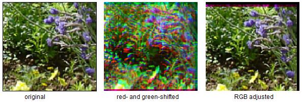
Adjust RGB
If one or two colour components is/are shifted with respect to the others, this menu item can seek the shift by cross-correlating the red, green and blue components in order to annul the shift. Note that the borders of the final "RGB-adjusted" result need trimming. This menu option is the automated variant of the manual layer shifting tools     in the drawing tool box.
  

Thresholding
In the dialogue window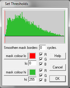 that pops up after selecting this menu item, a graph representing the "intensity density histogram" is shown along with two vertical lines. The density histogram shows how often pixels of a certain intensity (i.e. the sum of red, green and blue pixel values, if selected) appear in the bitmap. In the histogram, intensity runs from left to right. The two vertical lines, that indicate the lower and upper thresholds, can be moved by dragging them with the mouse to the left or to the right. Pixels having intensities below the lower threshold or above the upper threshold will be replaced by the mask colour shown underneath the histogram. The mask colour may be changed by pushing the "mask colour" button. In that case a second dialogue window pops up, showing a palette from which a new colour may be chosen. This menu item is enabled only if a single bitmap object is selected.

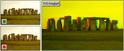
Anaglyph/Merge
Anaglyph: Two bitmaps can be combined into either a red-green or a red-blue anaglyph. If the two bitmaps depict the same scene with a slight parallax, the resulting anaglyph will appear to be three-dimensional when viewed with red/green or red/blue glasses.

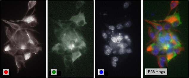
Merge: The red colour component of a bitmap may be combined with the green colour component of a second bitmap and the blue component of a third with the "RGB Merge" option. If the three bitmaps were obtained for example from the same histo-chemical preparation using three differently coloured marker dyes, one red, one green and one blue, the resulting image will show the three markers superimposed.

To select the bitmaps for the operation push the button in the "Set RGB bitmaps" dialogue window. Then push the button to indicate that the current bitmap will provide the "red" information. The button will change into , indicating that the currently displayed bitmap will be used for the red component. Proceed similarly for the "green" and/or the "blue" bitmap. Prior to combining the bitmaps, their contrast profiles may be changed. To do so, push the button. The "bitmap contrast" dialogue box, described above, pops up, showing the contrast profile used in the previous "anaglyph/merge" session. The profile is marked "Red", "Green" or "Blue", depending on the colour of the button clicked. The contrast option is active only if the box is checked.
Noise may be removed by checking the "rem noise" option.
The result, but not the original images will be affected by the contrast and noise options.
The same bitmap may furnish the red, green and blue components, allowing to modify the contrast of each colour component separately or to create special effects.
In case he original red, green and blue component images are shifted a few pixels with respect of one another, check the "Adjust RGB" box. Then the three images will be cross correlated and the shift will be compensated. This only works if the three images are not too dissimilar. This function resembles the Adjust RGB option from the Bitmap menu.
Per default, the program shows all images on all drawing sheets. Check the "List bitmaps of this sheet only" box if you wish to browse only the images on the currently active sheet.

Alpha merge
Alpha merging or alpha blending is the technique whereby the, usually homogenous, background of one image is replaced by the contents of an other image. To change the background of the image to the left below, slect the image and choose Alpha merge from the menu.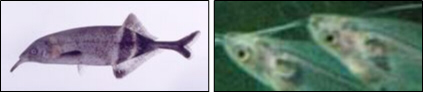

A dialogue box comes up to select the background colour. To do so either edit the R,G and B boxes, taking values between 0 and 255, or push the "pick colour" button. In the latter case the cursor changes into a pipette. The tolerance parameter determines the precision of the background mask. It may vary between 1 and 255.

Push "OK". In the next dialogue box, choose the bitmap to replace the background with. Then a new blended bitmap will appear on the drawing sheet.

Superimpose
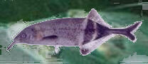
With this menu item the images of two or more bitmaps can be made exactly overlapping. It has been included in Cells&Maps to align time lapse images in order to create video animations. A practical example is probably the best way to illustrate its function: Images of growing young neurones were taken with a camera attached to a microscope with regular intervals (time-lapse). The microscope stage and the petri dish were moved in between images, which is the reason that the alignment of the four images shown below is far from perfect.

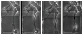
The three images to the right can be aligned to the leftmost image by selecting superimpose from the bitmap menu. In the dialogue box that pops up, the leftmost image was selected as the template and one of the other three as the overlay (below the result is shown if the third image from the left is chosen as the overlay). In this example red/green overlay has been selected in the dialogue box, meaning that the template image is represented as green and the overlay image as red. Other possibilities are 'average' (transparent), OR or XOR overlays.

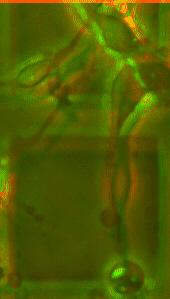
The mouse cursor has changed from arrow into . Now the red overlay can be moved using the mouse or the arrow keys on the keyboard. In order to rotate the overlay, press the <Ctrl> key, which changes the mouse cursor into . The centre of rotation will be in the centre of the image. After moving and rotating the red overlay the result may be as:

To terminate the alignment click on the arrow tool in the drawing toolbox. The red/green image disappears and the image selected as the overlay image will change into:

Here the bottom and right borders of the bitmap are white, but an other colour might have been chosen in the overlay dialogue box by pushing the 'fill colour' button. Doing the same for the other two remaining images results in:

To remove the white borders select all four images and use the align tool to stack the four images on top of each other, then use the cut tool to dissect the four centre parts of the images simultaneously:

To give a rough idea of cell movement use the anaglyph/merge item from the bitmap menu to combine for example the three images to the right into:

Count pixels
First select a bitmap and then count the number of pixels in the bitmap that are above or below a certain threshold. In order to select only pixels within the boundaries of a polygon, a square or an ellipse, select two objects, 1) a bitmap and 2) a polygon, square or ellipse prior to executing the Bitmap>Count pixels command. In the dialog box that comes up select either 'entire bitmap' or 'current polygon'. The routine returns a single number if 'grey scale' is selected, while it returns three numbers, one for each of the red, green and the blue components of the bitmap if 'Split RGB' is selected. With 'weigh intensity' each count is multiplied with the pixel intensity, hence a white pixel above threshold counts for 255 and a black pixel for 0 if pixels above threshold are counted. A black pixel below threshold counts for 255 and a white pixel for 0 if pixels below threshold are counted. With 'weigh intensity' unchecked, each pixel above/below threshold counts for 1. Set the threshold (0...255) with the slide bar or the edit box .

Count objects
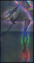
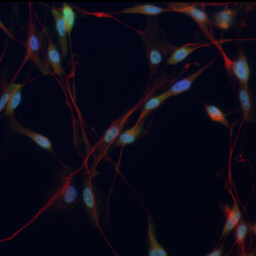
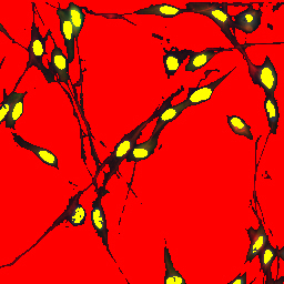
This menu item has been made with automatic cell detection and counting in mind, but it should also work with other kinds of objects. Its function is possibly best explained with an example: We would like to know how many cells are present in the figure below.

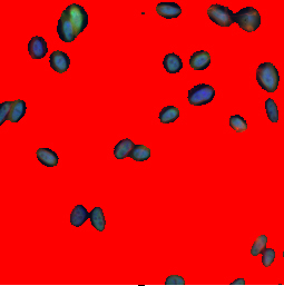
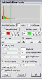
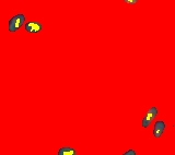
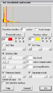
Some objects are well separated, but not all of them. Now we have to indicate where the nuclei centres are located. For this the green line is used, but because green shows not well on blue we change the colour first to yellow using the "nucleus colour button". Then we try to obtain a yellow spot at each nucleus centre.

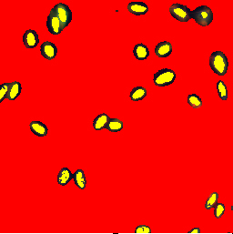
Set the yellow threshold such that each nucleus contains not more and not less than one yellow spot. Then push the OK button.
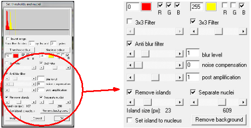
Several options present in the dialogue box are shown enlarged to the right. For the low (mask) and high (nucleus) thresholds 3x3 filters may be used that may be low-pass or high pass, depending on the position of cursor in the slide bar (middle position is no filtering). The anti-blur filter only applies to the mask and can not be used at the same time as its 3x3 filter. This filter inverse-filters blur coming from out-of-focus parts of the image. Normally inverse filtering requires knowledge about the so-called point spread function of the optical equipment (a microscope in this example). Since the point spread function is not known to XLPlot, it needs to be guessed by setting the "blur level" and "post amplification". Overestimation of blur may lead to a noisy image and therefore a dotted mask. This can be partially be undone with "noise compensation".
Sometimes objects may be partially covered by small patches (islands) of mask. Use "remove islands" to remove these patches. The slide bar setting determines the maximum size of the islands to be removed.
Nuclei that are supposed to be separate, but have become fused may be separated using "separate nuclei".
When "Remove background" is clicked, the average red, green and blue values of the pixels under the mask are subtracted from the bitmap. This is especially useful for the Object properties option below that uses the same dialogue window.
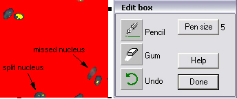
Finally, manual editing may be necessary for certain images to label missed nuclei, to fuse split nuclei or to separate fused nuclei. The pencil in the dialogue box below will draw a yellow line. The gum will draw a black line. In the example below at the left, a nucleus has been missed and another has been split into three small ones. This has been corrected at the right using the pencil. Use the "Undo" button to start manual editing all over again.

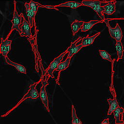
After having pushed the "Done" button and after some calculation, the image changes again and a new dialogue box comes up:

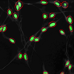
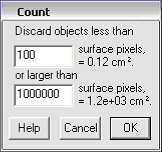
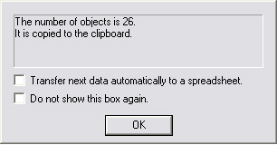
Each object is indicated by red borders, in the centre of which is a green dot that corresponds to the yellow dot of the previous image. Very small objects due to noise in the image may be generated. These can be removed from the count by setting a lower limit for the surface of objects. The surface to be entered in the edit box is in pixels. The surface in square centimetres is shown to the right of the edit box assuming a resolution of 72 pix/inch. When done, push the OK button. A third dialogue pops up with the result of the count. If you wish the result to be added to the bottom line of a spreadsheet check the "Transfer next data automatically to a spreadsheet" check box.

The "Set threshold and nuclei" dialogue box (the first one that came up) contains a few options that were not explained yet, as they were not needed in the example above. With "Smoothen mask borders" the occurrence of objects with a size of one or just a few pixels can be prevented.   

A comprehensive demo of which the spoken text refers to Finnegans wake by James Joyce: "Object properties" should be viewed full screen Object properties
Please read the Count objects section first before proceeding. In contrast to the section above, we do not merely wish to count the number of nuclei, but we also wish to know the size and the amount of red labelling (actually red fluorescence in this example) of each cell. Now the threshold mask is set taking into account all three, R,G and B, components such that the cell contours are delineated. The nuclei are selected using only the blue component.

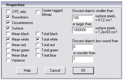
Then after possible manual editing, the "Properties" dialogue box appears (middle figure below). The properties we wish to determine for each cell may be selected in this box. Most options are fairly self-explanatory: The "Circumference" and "Surface" options measure the circumference (in cm) and surface (in cm²) of each cell assuming a 72 pixels/inch (28.3 pixels/cm) image resolution. "Mean intensity" measures the brightness of each cell, which may vary between 0 (black) and 255 (white). Similar for "Mean red", "Mean green" and "Mean blue". If the "variance" box is checked, the variances for "intensity", "red", " green" and " blue" are calculated. The "Roundness" option calculates, using principal component analysis, the sizes of two perpendicular vectors in 2D space and then takes the ratio of the sizes of the two vectors. This ratio is a measure of the roundness or elongation of the cell. A circle gives two vectors of equal size and hence a ratio of one. An ellipse has a ratio of less than 1. A needle has a ratio of almost zero. The "2PC ratio" option forms vectors taking into account the red, green and blue intensities and the x an y positions of each pixel belonging to a cell. Then the ratio of the two first principal components is computed. Although the physical interpretation of the result may not always be clear, it helps to find out whether differences amongst cells exist, whatever those differences might be.
After pushing the "OK" button, the data are transferred to a spreadsheet. If the "Create tagged bitmap" box was checked, a new bitmap (not necessarily of the same size) is created, with which the new data is associated.

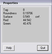
If you select the "tagged" bitmap and then select the pipette tool , then the "Properties" dialogue box shown are the right above comes up. If the pipette is over a bitmap tag, the dialogue box shows the properties of the object. The pipette tool fulfils its original mission if you click the left mouse button, that is: it finds colour index belonging to the pixel.

Get mean background
Select both a bitmap and a polygon (any closed figure, such as a rectangle) and then issue the Bitmap>Get mean background command. XLPlot will determine the mean RGB intensities of the bitmap pixels that are within the polygon. These values can be subsequently used to carry out thresholding and background subtraction. The value may also be copied to a spreadsheet.

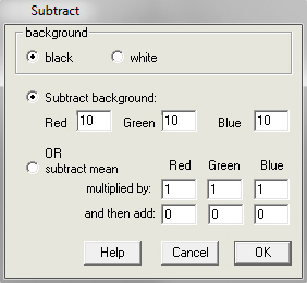
Subtract background
With this menu item you may subtract a constant value from all pixels in the currently selected bitmap. In the dialogue window that pops up, chose either "Subtract background", which will subtract the RGB values shown in the edit boxes , or "Subtract mean", which will subtract the mean pixel intensity in the whole bitmap from all pixels. The value shown in the "subtract background" edit boxes may have been obtained previously using the Get mean background command. When using the "subtract mean" option, the RGB values to be subtracted may be first multiplied by a factor shown in the second row of edit boxes (1 per default). After subtraction a constant value as entered in the lowestrow of edit boxes may be added (0 per default). You set the colour of the background (black or white) in the upper panel.

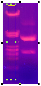
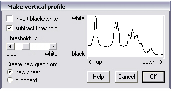
Vertical profile
The optical density profile of a for instance a migration gel can be created using this menu item. Draw a rectangle on the image of the gel, select both image and rectangle and issue the Bitmap>Vertical profile command. A dialog window will pop up. Use the horizontal scrollbar to set the background level that will be subtracted from the image. When using the Get mean background command from the bitmap menu before using the vertical profile command, the threshold shown in the dialogue box is equal to the mean background. A preview of the graph that will be created upon pushing the OK button is shown in the right hand panel.

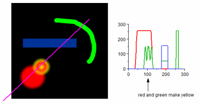
Line profile
The red, green and blue pixel intensity profiles on a straight line drawn over a bitmap are obtained with this menu item. Select both a bitmap and a straight line, issue the command from the menu and a new drawing sheet with a single graph showing the red, green and blue profiles will appear. The ordinate indicates pixel intensity (from 0 to 255) and the abscissa is in pixel number starting at left-most point on the line over the bitmap. In the example below the line first crosses a red circle, then two yellow-orange concentric circles followed by a cyan-blue block and a green squibble.

 UP↑

Insert bitmap in bitmap
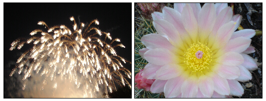
If you wish to insert a bitmap image into another bitmap, proceed as follows. Suppose your drawing sheet contains the two bitmaps below and you wish to insert the flower into the fireworks.

Resize the bitmaps and arrange them such that the flower is inside the fireworks photo:

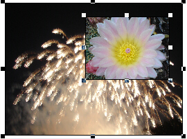
select both bitmaps and issue the Insert bitmap in bitmap command. A new bitmap will be created that contains the flower as an insert in the fireworks bitmap.

Cut out a rectangle
Select or draw a rectangle object onto a bitmap and issue this command. A section corresponding to the rectangle will be copied from the bitmap.

Reduce number of colours
A dialogue box requesting the number of colours will appear:

The number of colours may vary between 2 and 256. The resulting bitmap will be a colour-indexed, i.e. a bitmap that refers to a palette to define its colours. If you leave the "Impose the currently active palette" box unchecked, a new palette will be calculated for the bitmap. If you choose to impose the currently active palette, then the bitmap will use the currently active palette. The currently active palette is the palette that is associated with the drawing sheet. This palette may be changed using the Tools>outline colour, Tools>fill colour or the Tools>Get palette from bitmap menu items. As the first three colours of the palette have a special meaning for the drawing sheet (transparent, background and foreground colour), they will not be used to create the new bitmap. The first usable colour index starts at 3 (the 4th colour box in the palette). Note that if you use less than 256 colours, for example 4, then only the colours 3 through 7 will be used. This will be 3 through 19 if you choose 16 colours, etc.

half size
This menu item reduces the horizontal and vertical resolution of the currently selected bitmap by a factor of two.

Size to power of two
Several menu items (e.g. Bitmap math>Lorentzian filtering, (de)convolution and Bitmap>Object properties) carry out calculations that require Fourier transformationAny signal may be considered as a sum of sines and cosines of different frequencies and amplitudes. The Fourier transform is an algorithm that calculates the amplitudes as a function of frequency. The result is a series of cosine coefficients (the so-called real part) and a series of sine coefficients (the imaginary part). The frequency spectrum plots as a function of frequency, where R and I are the cosine and sine coefficient respectively. of bitmaps. If the dimensions are powers of two then Fast Fourier transformation (FFT) can be used as opposed to regular Slow Fourier transformationAny signal may be considered as a sum of sines and cosines of different frequencies and amplitudes. The Fourier transform is an algorithm that calculates the amplitudes as a function of frequency. The result is a series of cosine coefficients (the so-called real part) and a series of sine coefficients (the imaginary part). The frequency spectrum plots as a function of frequency, where R and I are the cosine and sine coefficient respectively. (SFT). Depending on bitmap size, the difference in calculation time may be very large: a 1024x1024 image was transformed in 100 ms on a Intel 2.8GHz 2 Quad computer, while a 1023x1023 image took 1 minute to transform; 600 times as long. The difference grows with increasing bitmap size. It may therefore save time if the images to analyse are converted to images having dimensions of powers of two. After having chosen this menu item, the "Powers of two" dialogue pops up presenting three sizing options: "Decrease" the size of the bitmap to the next largest map with power of two dimensions, "Increase" the size or choose "Optimal". The last option finds dimensions that most closely match the original dimensions.

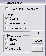
If the "Stretch to fit new bitmap" box is checked, then the original image will be deformed to fit the new image. Deformation may not always be a problem. It isn't for example if one only wishes to count the number of objects in an image that needs filtering. If the "Stretch to fit new bitmap" box is not checked then part of the new bitmap contains undefined pixels that need to be attributed the background colour. Use the "Border colour" options to choose between black or white background or let the program find the average colour of the pixels on the map border (Automatic).

Copy window as bitmap
The current window or the entire drawing sheet is copied to the clipboard in windows bitmap (*.BMP) format when selecting this menu item. The resolution can be chosen in the dialogue box that will pop up. The contents of the clipboard may then be pasted in a program that accepts bitmaps (photoshop, corel photopaint etc.) for further modification.

Slide show
You can show your bitmaps at full screen using this option. The bitmaps should reside in a single folder, on a drawing sheet or their location should be specified in a text file. You can set the interval between successive slides in the dialogue window that comes up. If you have a second display monitor then you can choose to alternate between the two displays. The resolution of the two displays need to be identical. Type the <escape> key to quit the slide show. If you specify the location of the bitmap files in a *.txt file, please observe the following rules (see the figure below). The text file should be in tab-delimited format, just as the programs spreadsheet format. The first column should contain the path to the bitmap, the second and third columns are optional and specify the monitors on which the bitmaps should be displayed. 1 is for the principal monitor and 2 is for the auxiliary monitor. The third column specifies the time in ms until the next slide. Note that the file should be saved in TXT and not in ETF format.

Show all dialog windows
Several dialogue boxes contain the option "do not show this box again (during this session)". In order to make those boxes reappear again next time, issue the Show all dialog windows command.

The Bitmap Math menu

Histogram
First select a bitmap and then create a probability density histogram of pixel intensity with this menu item. In order to select only pixels within the boundaries of a polygon, a square or an ellipse, select two objects, 1) a bitmap and 2) a polygon, square or ellipse prior to executing the Bitmap>Histogram command. In the dialog box that comes up select either 'entire bitmap' or 'current polygon'. The routine returns a histogram that contains a single curve if 'grey scale' is selected, while it returns three curves, one for each of the red, green and the blue components of the bitmap if 'Split RGB' is selected. The histogram is copied to a new document or to the clipboard. If the latter option is selected, nothing seems to happen until a paste command is issued. With 'invert bitmap colours', left and right are inverted in the histogram. With 'integrate histogram', the data in the histogram are integrated from left (x=0) to right (x=255).

Bitmap math
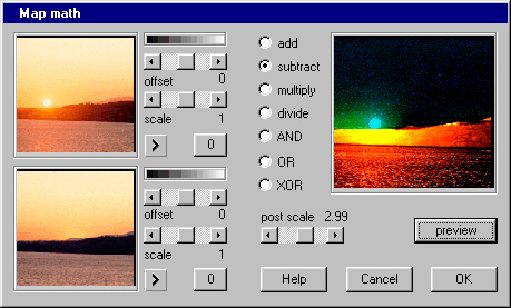
A few basic mathematical operations (addition, subtraction, multiplication, division, ANDing, ORing and XORing) can be carried out between two bitmaps using this menu option. After selecting the Bitmap math menu item, a dialogue window pops up. Use the buttons to choose the images. Per default, the program shows all images on all drawing sheets. Check the "List bitmaps of this sheet only" box if you wish to browse only the images on the currently active sheet. Offset and intensity amplification of the starting images can be set with the horizontal slide bars. Above the slide bars, a grey scale is shown to give an idea of how the colour distribution of the image will be affected. Click the button to reset the offset and scale to default (0 offset, scaling 1). After the addition, subtraction, multiplication or division of the two bitmaps, post-amplification can be carried out with the slide bar "post scale" slide bar. Pushing the "preview" button will show the result. Bitmaps of unequal sizes will be aligned at the top left corner.

Average bitmaps
Sometimes, it can be useful to eliminate noise by averaging several images taken of the same scene or to correct background illumination by subtracting an averaged reference image from a scene. With this menu item it is possible to average a number of images that were previously imported onto the program's drawing sheets. The selection of bitmaps to average is made with the dialogue window that comes up after issuing the Average bitmap command. Use the "Add" button to add an image to the list of images to be averaged and push "next" to proceed to the following image. If the image currently displayed is already in the selection list, the "Add" button will transform into a "Remove" button such that the image can be removed from the list. The program shows all images on all drawing sheets. Check the "List bitmaps of this sheet only" box if you wish to browse only the images on the current, active, sheet. Bitmaps of unequal sizes will be aligned at the bottom right corner and will probably give unwanted results.

Correlate colours
With this option the pixel by pixel correlation between intensities of two of the three colours (R,G,B) making up a bitmap are calculated. A correlation coefficient between -1 for perfect negative correlation and +1 for perfect positive correlation is returned. It is meant to estimate co-localisation of two proteins each labelled with a different colour. When selecting this menu item, a dialogue box pops up allowing for setting lower and upper thresholds, thus eliminating certain regions from analysis.

Filter
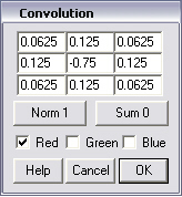
For Lorentzian filtering, see the next section on Fourier transformation first. With the Filter>3x3 matrix Convolution item an image is convolved with a 3x3 matrix of the users choice. In the example below, the image to the left was convolved with a differentiating matrix resulting in the image to the right. It enhances borders of objects in the image because the centre of the convolution matrix is of opposite sign as its borders. The sum of the border cells is identical to the centre value and hence the sum of all nine cells amounts to zero. When pushing the "Norm 1" button, the content of all the cells will be scaled such that the sum of all cells amounts to 1 (Normalisation to 1). When pushing the "Sum 0" button, the value of centre cell will be recalculated such that the sum of all nine cells is zero. Convolution is carried out for the red green and blue component separately.

Filter>Anti blur filter
Images that are somewhar blurry may be sharpened by estimating the point-spread funtion and then deconvolving the image with that function. As generally speaking we do not know what the point-spread function really is, an exponentially decaying function around the centre pixel is assumed. Set the point-spread constant (filter constant) in the dialogue box that appears (0.2 in the example shown below). The higher this constant the farther the centre point spreads out. Note that noise and imperfections in the image are also deconvolved leading to still more noise in the resulting image. One way to counter this phenomenon is to carry out noise removal before and after deconvolution.

Filter>Lorentzian low-pass and high-pass filters
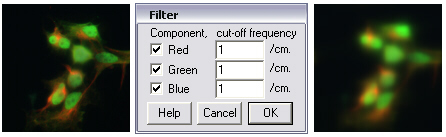
When applying the Filter>Lorentzian low-pass filter to a bitmap, Fourier transformationAny signal may be considered as a sum of sines and cosines of different frequencies and amplitudes. The Fourier transform is an algorithm that calculates the amplitudes as a function of frequency. The result is a series of cosine coefficients (the so-called real part) and a series of sine coefficients (the imaginary part). The frequency spectrum plots as a function of frequency, where R and I are the cosine and sine coefficient respectively. (FT) is first carried out, then the spectral components are adjusted according to a Lorentzian function and finally the inverse FT is carried out. A Lorentzian is the power spectrum of an exponential function |FT[exp(-kt)]|² = 1/(k²+ω²). k is the corner frequency (3dB point). In the figure below, the leftmost image was low-pass filtered with a spatial cut-off frequency of 1 period per cm. (again, 72 pixels/inch are assumed). Lorentzian high-pass is carried out similarly

With the Filter>Filter with template's spectrum, spectral components that are (almost) absent in the template used in convolution and deconvolution as described below are suppressed in the image. This might help remove noise in deconvolutions.

Fourier transformation
The application of the more simple one dimensional Fourier transforms can be found in the spreadsheet section. Just as a single one on a background of zeroes gives a "white" spectrum in the one-dimensional case, a single white dot against a black background gives a white two-dimensional spectrum. In the figures below the images in the upper row are converted into the spectra in the lower row. The latter should be read as follows: Zero frequency, f(0,0), is in the lower left corner of the spectrum's image. The images below are 128 by 128 pixels. Therefore th upper right corner represents f(64,64). Colour intensity is a measure of the energy contained in a particular frequency component. The pixel intensity is a logarithmic function of the spectral amplitude. This function, which takes into account the number of spectral components (and hence bitmap size), has been chosen to optimise visual information. After Fourier transformationAny signal may be considered as a sum of sines and cosines of different frequencies and amplitudes. The Fourier transform is an algorithm that calculates the amplitudes as a function of frequency. The result is a series of cosine coefficients (the so-called real part) and a series of sine coefficients (the imaginary part). The frequency spectrum plots as a function of frequency, where R and I are the cosine and sine coefficient respectively., the real and imaginary parts of the spectrum are stored in floating point format and remain associated with the bitmap, such that next manipulations, such as back transformation remain possible. This would not be possible when relying only on bitmap information (lack of numerical resolution). If the user manipulates the bitmap with procedures such as contrast enhancement or smoothing after having Fourier transformed the image, then the hidden floating point data and the bitmap do not correspond anymore and therefore the floating point data is removed. Fourier transformation works the fastest with bitmaps that have dimensions that are a power of two (e.g. 512 by 256, 1024 by 4096). Although Fourier transformation in this software has been programmed for multiple processors, calculation for bitmaps with other dimensions than power of 2 may take (too) much time. The larger the bitmap the bigger the difference between fast and slow Fourier transformation. A bitmap of 1023 by 1023 pixels takes 600 times longer to calculate than a 1024 by 1024 bitmap. You might want to use the Size to power of two item from the Bitmap menu to change image dimensions first.

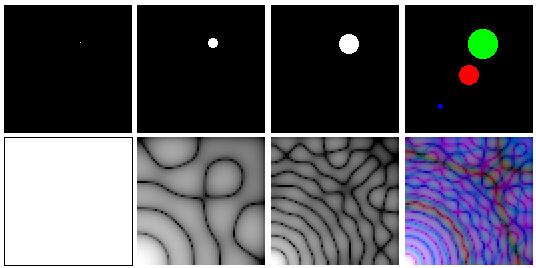
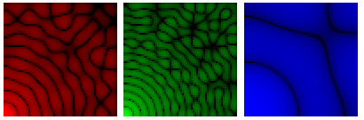
If one takes an image with a white dot larger than a single pixel on a black background (2nd from the left), then the spectrum contains hills (white) and valleys (black). The larger the dot, the closer the spacing between hills in the frequency spectrum. The rightmost image contains three coloured of different size. The corresponding spectrum is not easy to interpret: the spacing between red bands seems to be larger than the spacing between blue bands. Perhaps one would expect the opposite, because we just saw that smaller dots give wider interspaces. However if the spectrum is separated into red green and blue components the reason for this becomes clear: the red bands appear where there are dark bands in the green and blue spectra.

Set as template
Set the current bitmap as the template (form to be detected in an image) for (de-)convolution.

Convolve with template
After having set the template, an image can be convolved. The template image as large as or smaller than the image to be convolved. In the figure below, the first image has been convolved with the second image, resulting in the third, middle, image.

Deconvolve with template
The centre image in the figure above has been deconvolved with the template giving the rightmost image, which is more or less the same as the original image. Convolution and deconvolution of images in this software applies the convolution theorem, which states that the convolution of two functions is equal to the inverse FT of the product of the FTs of the two functions. Hence: f1 Conv f2 = FT^-1[FT(f1)*FT(f2)]. This means that (de-)convolution is carried out much faster if the dimensions of the images are powers of two. 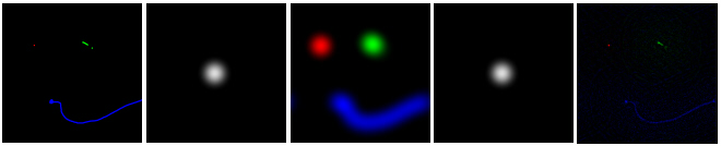Deconvolution is extremely sensitive to noise: the leftmost image below is the template, the second is the image to be deconvolved and the third is the result of the deconvolution i.e. a single dot where the centre of the where the object was.

After adding noise in the leftmost image below, deconvolution gives the second image from the left: just noise. Only after application of the Bitmap>remove noise three times to the original leftmost image is a more or less usable result obtained (rightmost image below).

The Stack menu

How to animate a stack of bitmaps.

When using this menu it is possible to sequentially display a series of time-lapse images, thus giving an impression of motion. The images have to be in uncompressed *.TIF or *.BMP format and reside all in the same folder. All their names have to begin with identical non-numerical characters and terminate in different numbers (e.g. "image01.bmp, image02.bmp"). The number of numerical fields in their names should be identical. Hence, image001.tif through image999.tif is OK, but image1.tif through image999.tif is not. 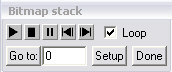The creation of an animation occurs in two steps: Step 1. Import one of the bitmaps of the series onto the drawing sheet and select it. A dialogue window appears alongside the tool window:

Step 2. If you then push the "Setup" button, the following dialogue box appears next to the drawing sheet:

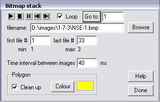
In this dialogue window you may modify several parameters if necessary. Enter another filename path, including the filename itself, in the edit box or push the "Browse" button. Modify the first and last file number of the series of images to animate in the "first file #" and "last file #" edit boxes. For example, if the image series runs from "boite001.bmp" to "boite100.bmp", these values are "1" and "100" respectively or any other pair of values between these limits with "last file #" greater or equal to "first file #". The animation is not interrupted if the image series contains a few gaps (i.e. some bitmaps are missing). Hence it not necessary to renumber the bitmaps after having removed an unwanted image. However, if the number of missing images exceeds 10, animation is stopped and "Error" is displayed in the "Go to" edit box. The time interval (in ms) between successive images is set in the lower edit box. As the Windows multitasking environment uses time slices of approximately 50 ms, values less than that are of little effect. With a slow computer and/or large image files, the actual delay may be larger than the one chosen by the user, as XLPlot does not skip images to compensate for time lost by processing images. Check the "loop" checkbox in order to replay the sequence continuously.
Press the play button to start the animation.
Stop animation.
Pause/resume animation.
If stopped or paused, pressing this button loads the next image in the range. XLPlot will not load an image number larger than "last image #", even if it exists. Pressing the "n" key on the keyboard has the same effect, provided that the drawing sheet containing the bitmap object has the input focus (i.e. the drawing sheet is the "active" window).
If stopped or paused, pressing this button loads the previous image in the range. XLPlot will not load an image number smaller than "first image #", even if it exists. Pressing the "p" key on the keyboard has the same effect, provided that the drawing sheet containing the bitmap object has the input focus. In order to display image number "x", type the desired number in the "Go to" edit box and press the "Go to" button.

A polygon may be traced onto the animated bitmap to depict the path followed by a moving object. In order to do so, go to the first image in the sequence, activate the drawing sheet and right-click once on the object to follow. A coloured dot appears on the bitmap. Then push the "n" key on the keyboard to load the next image and right-click again on the object that may have changed position. The dot is now replaced by the first segment of a polygon. Push "n" again and continue constructing the polygon until the last image in the sequence is reached. Rather than continuously switching between keyboard and mouse, one may move the mouse pointer on the screen by using the arrow keys and press the "h" key to emulate a mouse click. Using the arrow keys in combination with the (Ctrl) key moves the pointer 10x faster. Left-click anywhere to finish the polygon. See polygon tracking for a very similar function.

Add, Subtract, Alpha merge, AND, OR, XOR a bitmap
With this menu item a bitmap can be added to, subtracted from, Alpha merged with, ANDed ORed or XORed with a stack of numbered bitmaps. To do so, a bitmap of identical dimensions as the bitmaps in the stack needs to be present on the drawing sheet. For example to subtract a background image from all the images of the stack, import the background image and one image from the stack onto the sheet. Select the stack image and issue the Stack>subtract bitmap command. A dialogue window will appear with which you can browse through the images currently imported by the program. Push the "select" button when you have found the background image that you wish to subtract. After that, a second dialogue window pops up that allows you to modify the range of images to subtract from and the prefix of the filenames that will contain the result. Per default the same prefix as the source filename is suggested, which will result in the source files to be overwritten. Change the prefix if you do not want this to happen.

Stack > .....
The other functions listed under the Stack menu e.g. "smooth", "remove noise" etc. work similarly. Smoothing, noise removal, a previously recorded macro or one of the other functions is carried out on each of the bitmaps in the numbered list (stack) and the modified bitmaps are then written to hard disk. An exception to this rule is Stack>count pixels, where nothing is written to disk. The results of the pixel counts on each of the bitmaps in the list appear on a spreadsheet. A dialogue window pops up that allows you to modify the range of images to subtract from and the prefix of the filenames that will contain the result. Per default the same prefix as the source filename is suggested, which will result in the source files to be overwritten. Change the prefix if you do not want this to happen.

Add, Alpha merge, AND, OR, XOR a stack
Whereas the above discussed operations take a single bitmap stack as an argument, the Add a stack, AND a stack etc take two stacks as arguments. Say, you have two stacks, StackA and StackB. Select the two stacks by clicking on both of them while maintaining the <Shift> key depressed. Then, after issuing for instance the XOR a stack command the following dialogue window comes up:

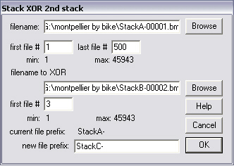
The names of the two source stacks may be modified using the "browse" button. The names of the two stacks may be identical. The new file prefix should be chosen as, per default, it is identical to the first stack name. Hence if you do not change the prefix, the original bitmaps will be overwritten. Set the first and last bitmap number of the stackA to be processed and set the first number of stackB. In the above example the first bitmaps to be XORred will be StackA-00001 and StackB-00003, followed by StackA-00002 and StackB-00004 etc. until StackA-00500 and StackB-00503.

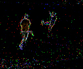
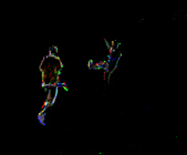
Differentiate
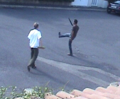
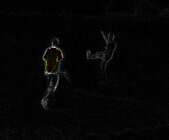
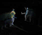
With Stack>Differentiate you may create a series of bitmaps that depict the differences between successive images in a stack of images. Concretely: The leftmost image below shows one image in a stack of images that were taken with a video camera. After calculation of the difference with the preceding image, the image in the middle is obtained. All pixels that do not change in between successive images become black. Hence the background (car, tiles) disappears and only movement remains. The rightmost image is obtained by selecting the 'trail' option in the Differentiate dialogue box and choosing a trail length of 20 images. This means that the contribution of a particular input image remains present in the resulting output images with a half life-time of 20 images.

The same dialogue box also offers the possibility to carry out XOR or NAND operations instead of differentiation between successive images. Each pixel in the image is colour coded by 3x8=24 bit, 8 bit for red, 8 for green and 8 for blue. The XOR and NAND operations consist of a bit wise operation between the corresponding bytes in two images. For instance if the red component of a pixel in image X is 10010110 (150) and the corresponding component in image X+1 is 10010101 (149), the XOR result will be 00000011 (3). Logical operations between images will often give rise to considerable noise in the output image, since small variations in pixel intensity may have large effects. Consider for example the XOR result of 128 (10000000) and 127 (01111111). The difference is only 1 but the XOR result is 255 (11111111). The dialogue window proposes to apply a threshold below which the XOR (or NAND or differentiate) operation will not be carried out and the output pixel colour component will be assigned the value 0 (black). However, even then noise may not be completely suppressed and a few specs may still show up in the output image. It can be cleaned up by checking the 'remove noise' option (lower right).

Cut out
If you wish to cut out a rectangular section of each of the bitmaps in a numbered stack of images: 1) Draw a rectangle onto the bitmap. 2) select both the image and the bitmap. 3) Issue the Stack>Cut out command. A Dialogue window comes up prompting for the range of files (starting number and final number) and the new file prefix. Per default the prefix is identical to the source, which means that the source file will be overwritten by the result file. Do not forget to check the "Save file to disk" box, otherwise nothing will be saved on disk.

Bitmap in bitmap
With this menu option you can insert a stack of images into a fixed bitmap or, inversely, insert a fixed bitmap into each bitmap of a stack. See the bitmap in bitmap option in the bitmap menu for how to proceed.

Number of colours
The maximum number of colours in each bitmap of a stack of bitmaps will be modified using this menu item. First, a dialogue box asking for the range of bitmaps and the filename prefix will pop up. Do not forget to check the "Save files to disk" box. Second, a dialogue box requesting the number of colours appears:

The number of colours may vary between 2 and 256. The resulting bitmaps will be a colour-indexed, i.e. a bitmaps that refer to a palette to define their colours. If you leave the "Impose the currently active palette" box unchecked, a new palette will be calculated for each bitmap in the stack. If you choose to impose the currently active palette, then all bitmaps in the stack will use the currently active palette. The currently active palette is the palette that is associated with the drawing sheet. This palette may be changed using the Tools>outline colour, Tools>fill colour or the Tools>Get palette from bitmap menu items. As the first three colours of the palette have a special meaning for the drawing sheet (transparent, background and foreground colour), they will not be used to create the new bitmap. The first usable colour index starts at 3 (the 4th colour box in the palette). Note that if you use less than 256 colours, for example 4, then only the colours 3 through 7 will be used. This will be 3 through 19 if you choose 16 colours.

Save as jpeg
The stack of bitmaps (in bmp format) will be saved as a stack in jpeg format.          Create animated Gif

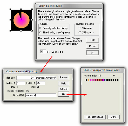
A stack of numbered bitmaps can be converted into a animated gif with a transparent background colour (black in the example above). To do so, load any image from the stack on the drawing sheet. For this example it was the second image. Then issue the command: Create animated gif from the Stack menu. In the first dialogue box that appears, select the colour depth (16 or 256) and the time interval between images in units of 10 ms (it will be 100 ms or 1/10th of a second in this example). A single (global) colourtable will be applied to all of the images in the stack (in contrast to accompany each image with its own colourtable, which makes the final gif file voluminous). So if an image in the stack would have contained blue or green shades, it would have been a problem basing the colourtable on only the image loaded on the drawingsheet. It is possible to prepare a colourmap beforehand using the drawingsheets palette, which can be edited with the options: Tools>outline colour, Tools>Fill colour and Tools>Get palette from bitmap. Then click OK. In the second dialogue box, the number of images, the starting and final image and the name of the giffile (animation.gif in this example) can be chosen. The extension ".gif" will be added automatically. The transparent colour index can be chosen in the third dialogue box. When you press the "pick from bitmap" button, the cursor changes into a pipette. Then click on the bitmap and the corresponding index will appear in the box.

          

Z voxels
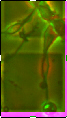
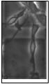
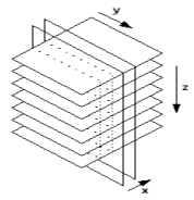
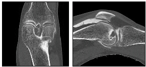
If a stack of images is available representing slices of an object, that has been sliced along, say, the z axis, then new stacks can be generated that represent the same object but now sliced along the x or y axis. In the following example a leg has been scanned by low dose X-rays at the level of the knee giving rise to 192 images representing transverse slices of the leg of which three are shown below:

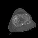
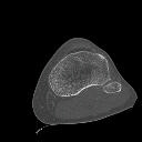
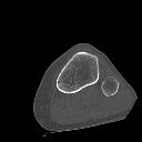
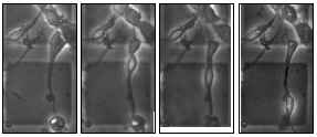
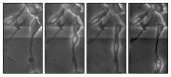
After running the Stack>Z voxels item new stacks are generated that give views that are perpendicular to the original views.

Size to power of two
Several menu items (e.g. Bitmap math>Lorentzian filtering, (de)convolution and Bitmap>Object properties) carry out calculations that require Fourier transformationAny signal may be considered as a sum of sines and cosines of different frequencies and amplitudes. The Fourier transform is an algorithm that calculates the amplitudes as a function of frequency. The result is a series of cosine coefficients (the so-called real part) and a series of sine coefficients (the imaginary part). The frequency spectrum plots as a function of frequency, where R and I are the cosine and sine coefficient respectively. (FTs) of bitmaps. FTs are carried out much faster if the bitmap dimensions (in pixels) are powers of two. It may save time if the images to analyse are converted to images having dimensions of powers of two beforehand. For more information consult the Bitmap>Size to power of two section. In the dialogue box that pops up, enter the path to the first image of the series (or push the "Browse" button), set the first and last image number of the series to convert and choose a new prefix for the reduced bitmap files. The prefix is the non-numerical part of the filename. The new files will be written in the same folder as the current files. The new prefix may be identical to the current prefix, in which case the original bitmaps will be overwritten.

Half size
Animation speed may be compromised if the bitmaps are large. Hence, one way to increase speed is to reduce the sizes of the bitmaps. This menu item reduces the bitmap sizes of the whole animation series by a factor of 2. In the dialogue box that pops up, enter the path to the first image of the series (or push the "Browse" button), set the first and last image number of the series to convert and choose a new prefix for the reduced bitmap files. The prefix is the non-numerical part of the filename. The new files will be written in the same folder as the current files. The new prefix may be identical to the current prefix, in which case the original bitmaps will be overwritten.

File rename
This menu item allows you to rename numbered bitmap files (stack), either by modifying numbers at the end of the file names or by replacing a sequence of characters in the name by another one. The "Rename files" dialogue box is divided in two. In the upper part one may increase or decrease the file number by a constant value. XLPlot will search for filenames that begin with the string entered in the "Filename prefix" edit box. Hence "Afile_A_01.bmp" and "Afile_B_01.bmp" may both be renamed if the prefix is "Afile" but "AAfile_A_01.bmp will not.

The Macro menu

If the same set of actions has to be carried out repeatedly on multiple drawing objects, then it may be useful to record these actions using the Start and Stop recording commands from the Macro menu. Once recorded, the sequence of commands constituting the macro can be rerun on other objects using the run macro command. For the time being the possibilities of the macro function are rather limited and concern only the actions that require a single (bitmap) object such as remove noise, adjust contrast etc. Indeed, the main reason why the macro function is included in the program is to facilitate bitmap stack operations and thus to prevent RSI (repetitive strain injury, due to too much mouse clicking). After having selected a single drawing object and having issued the start recording command from the Macro menu, only those menu items that can be recorded are enabled. The bitmap math item from the Bitmap Math menu for example, will be disabled because it requires two bitmap objects as input.

Manuals