The drawing sheet
Importing NCBI heatmap data
If you know the NCBI's GDS heatmap number, for example if you have been browsing the geo profiles database, then you may directly download the heatmap onto the drawingsheet using the Import from NCBI option from the Heatmap menu.
Type the number after 'GDS' in the dialogue box that appears and pusk 'OK'.
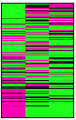
Heatmaps in Clusters may be created manually using the spreadsheet (the impractical way). The format has to be as in the figure below:

The upper row should contain labels identifying experimental conditions. The First column, "ID_REF", should contain references. When this version of Clusters was released, the program did not (yet) use this column, it is there mostly for compatibility with the NCBI heatmap format. The second column, "IDENTIFIERS" should contain gene labels, preferably using the official nomenclature (as the HUGO nomenclature for human genes). Clusters uses this column to search the NCBI database. Entries that do not comply with the official gene names, will be probably difficult to deal with. The rest of the matrix contains gene expression levels in floating point format. Once the spreadsheet is ready and the matrix selected, issue the Make heatmap item from the spreadsheet's Math menu.
A more practical way to create a heatmap is to download the data from the NCBI Geo profiles site:

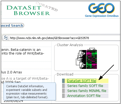
Search for the heatmap data you wish to import and click on the DataSet SOFT file link (and NOT the FULL.soft link if there is one):
Now there are three options:
1) If your browser asks for a program to open the GDSxxx.soft.gz file, you may select Clusters to do so. The heatmap will be automatically created on an open drawing sheet or, if it does not exist, a new one.
2) If you write the file to disk you can open the .gz file in Clusters using the File>Open option or by dragging the file onto Clusters. The .gz file will be uncompressed and a new file GDSxxx.soft will be created in the same directory. The heatmap will then be created on a new drawing sheet.
3) You may uncompress the .gz file by your decompressor (e.g. Winzip, gzip or 7-zip) and open the .soft file in Clusters. The heatmap will be created on a new drawing sheet.
Finally, if you know the GDS entry number, the data may be downloaded directly by the program using the Heatmap>Import from NCBI menu item.
The Bitmap menu
Import bitmapWindows bitmaps (*.BMP), uncompressed TIFF bitmaps and JPEG bitmaps may be added to the drawingsheet using this menu option or by pushing the
To restore the height/width proportion, double click on the image. In the dialogue box that appears, change the horizontal and vertical resolutions to identical values or click one of the buttons "1/8", "1/4" etc. The button "1" sets the horizontal and vertical resolutions to the monitor screen resolution of 72 pixels/inch. The button "1/2" sets the image size to half (144 p/i) etc. Most printers have at least a resolution of 600 pixels/inch.
A second way to import a bitmap is by copying it from a bitmap editor such as Photoshop and pasting it on the drawing sheet. If a 16 bit TIFF bitmap is imported, it needs to be converted to 8 bits. To minimise quality loss a dialogue box comes up requesting the range of intensities in the 16 bit bitmap to convert:

The dialogue box shows the darkest or lowest intensity encountered in the bitmap as well as the brightest or highest intensity found. These numbers can be edited, or the red cursors can be moved to change the settings.
Bitmaps can be exported similarly or by issuing the command Bitmap>Save bitmap or by pushing the ![]() button.
button.
Save bitmap
This menu option is enabled if a single bitmap object is selected. Select the bitmap format in the first dialogue window that pops up. Note that the 16-bit bitmap (32768 colours, a Windows 3.x format) is now almost obsolete and most bitmap programs such as Photoshop and Corel Photopaint will refuse to load it. Enter a file name in the next dialogue window that pops up. Note the difference with the menu item "Copy window as bitmap".
Bitmaps can also be saved by clicking the ![]() button or by pressing <Ctrl> S. While the menu selection prompts for the number of bitmap colours, the latter two actions assume the last used colour depth. Hence, these are shortcuts. Note that if no bitmap is selected, ^S will save the drawing sheet.
button or by pressing <Ctrl> S. While the menu selection prompts for the number of bitmap colours, the latter two actions assume the last used colour depth. Hence, these are shortcuts. Note that if no bitmap is selected, ^S will save the drawing sheet.
Size maps
With this option multiple bitmaps can be sized simultaneously. To do so, select the bitmaps to size and then issue the Size maps command from the Bitmap menu (or press <Ctrl> T). A dialogue box will pop up that allows you to choose between full size (1), one eighth, a quarter of or half the original size.
Note that bitmaps may also be sized as any other object, i.e. : Select the object. It has 8 little squares around it. If the mouse cursor gets over one of them it changes into a vertically, horizontally or a diagonally pointing pair of arrows. Depress the right mouse button and drag the pointer until the object has the appropriate size. Use the corner squares to change dimension in two directions and use the other squares to change size in one direction only. In order to maintain the original proportions of the object (x and y amplification identical), press the <Ctrl> key and release it after having released the mouse button.
A third way to size a bitmap is to double click on the image. In the dialogue box that appears, change the horizontal and vertical resolutions to the values of your choice.
Full screen
Use this option to display the currently selected bitmap full screen or type <Ctrl> O. Type the <escape> key to return to the program. If you have two display monitors, you may display a bitmap on the auxiliary monitor using <Ctrl> I.
Scale brightness
The colour of each pixel of a bitmap in this software is encoded by three bytes (a byte is a small integer number that can take on values between 0 and 255): one byte for the blue component, one for green and one for red. If the pixels in the bitmap have values that are all below 150 for example, then using Bitmap>Scale brightness>all multiplies all pixel values with a factor (255/150 in this case) such that the whole range of values between 0 and 255 is used. Whith using Bitmap>Scale brightness>Red only the red component is scaled. Scale brightness>Green and Scale brightness>Blue function similarly. Note that carrying out one after the other Scale brightness>Red, Scale brightness>Green and Scale brightness>Blue does not give the same result as Scale brightness>all, because in the latter case the scaling factor for all three components is the same and depends on the highest byte value found, irrespective of colour.
Adjust contrast
This menu option is enabled only if a single bitmap object is selected. The "bitmap contrast" dialogue box displays one out of five available response curves or "profiles" that determine how the intensity of each pixel in the bitmap will be modified when pushing the "OK" button. In the profile, current intensity runs from left (black) to right (white) and the new, modified, intensity runs from bottom to top. In order to increase contrast, choose a slope larger than unity. Inversely, to decrease contrast choose a slope less than unity. To invert the colours of an image choose a slope of -1. Other effects, such as solarisation, can be obtained with still other profiles, which may be of the user's design.
To go to the next or to the previous profile, push one of the ![]()
![]() buttons. To modify the current profile click on one of the nodes in the profile and move it up or down, while keeping the left mouse button depressed. By pushing the "default" button, the default profiles will be restored.
buttons. To modify the current profile click on one of the nodes in the profile and move it up or down, while keeping the left mouse button depressed. By pushing the "default" button, the default profiles will be restored.
Smooth
This menu option is enabled only if a single bitmap object is selected. The bitmap is passed through a 3x3-pixel (Gaussian) smoothing filter.

Original + noise Smoothing filter Median filter
Remove noise
This menu option is enabled only if a single bitmap object is selected. The bitmap is passed through a 3x3-pixel median filter.
Invert colours
The colours of the currently selected bitmap will be changed into their complements using this option. Hence yellow will turn blue and black will become white.
Pseudo colours
The colours of a bitmap may be replaced by a pseudo colour gradient. In the dialogue window, that pops up after selecting this menu item, the gradient is shown on the left and three sets of three slide bar![]() s on the right. With the slide bars the red (R), green (G) and blue (B) components of bottom, middle and top colours of the gradient can be set. The middle colour settings will be ignored if the
s on the right. With the slide bars the red (R), green (G) and blue (B) components of bottom, middle and top colours of the gradient can be set. The middle colour settings will be ignored if the ![]() box is unchecked. To see the effect of the settings on the currently selected bitmap check the "preview" box. Click "OK" to apply the pseudo colour gradient to the current bitmap.
If a pseudo colour gradient had been applied to the bitmap before, the text underneath the gradient shows "This bitmap has pseudo-colours". In that case, the gradient shown in the dialogue box corresponds to the current bitmap gradient rather than the default gradient. The default corresponds to the last gradient applied to one of the drawing sheet's bitmaps (allowing to apply the same gradient to multiple bitmaps) or, if none had been applied, the program default.
Pushing the "Make Bar" button creates a new bitmap object on the drawing sheet containing the gradient. This menu item is enabled only if a single bitmap object is selected.
box is unchecked. To see the effect of the settings on the currently selected bitmap check the "preview" box. Click "OK" to apply the pseudo colour gradient to the current bitmap.
If a pseudo colour gradient had been applied to the bitmap before, the text underneath the gradient shows "This bitmap has pseudo-colours". In that case, the gradient shown in the dialogue box corresponds to the current bitmap gradient rather than the default gradient. The default corresponds to the last gradient applied to one of the drawing sheet's bitmaps (allowing to apply the same gradient to multiple bitmaps) or, if none had been applied, the program default.
Pushing the "Make Bar" button creates a new bitmap object on the drawing sheet containing the gradient. This menu item is enabled only if a single bitmap object is selected.
The Heatmap menu
Heatmaps can be manipulated in several ways.
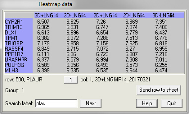
The first is to inspect the map and to localise gene entries in the map. To do this, select the heatmap first and then select the pipette tool ![]() from the toolbar. The dialogue box shown above on the right appears. When the pipette hovers above the map, a yellow square appears in the dialogue box indicating the entry that the pipette points at. The pipette can be moved one entry at the time by pushing the arrow keys on the keyboard. If the <Ctrl> key is held while pushing the arrow keys, the pipette moves half a page at the time. Use the page-up, page-down, home and end keys to move to the extremities of the data matrix. With a click of the left mouse button, a copy of the data shown in the dialogue box is made that can then be pasted on a spreadsheet. With the "Search label" edit box
from the toolbar. The dialogue box shown above on the right appears. When the pipette hovers above the map, a yellow square appears in the dialogue box indicating the entry that the pipette points at. The pipette can be moved one entry at the time by pushing the arrow keys on the keyboard. If the <Ctrl> key is held while pushing the arrow keys, the pipette moves half a page at the time. Use the page-up, page-down, home and end keys to move to the extremities of the data matrix. With a click of the left mouse button, a copy of the data shown in the dialogue box is made that can then be pasted on a spreadsheet. With the "Search label" edit box![]() and the "Next" button, text in the blue column and row can be searched. If a match is found, the pipette is repositioned on the map. Push the 'Send row to sheet' button to copy an entire row of data to a spreadsheet. The same can be done by right-mouse clicking on the spreadsheet and selecting 'Copy row' from the popup menu.
and the "Next" button, text in the blue column and row can be searched. If a match is found, the pipette is repositioned on the map. Push the 'Send row to sheet' button to copy an entire row of data to a spreadsheet. The same can be done by right-mouse clicking on the spreadsheet and selecting 'Copy row' from the popup menu.
Pushing the ![]() button will change the header to a header row that carries the group labels. Pushing it again will revert to GSM numbers. After a double-click in the upper left corner (labelled GDS3463 here), a text window containing the original GDSxxx.soft file header appears. This header may contain useful information about the experimental conditions. The header may also be invoked using the Data header item from the Heatmap menu. The dialogue box closes upon clicking "Quit".
button will change the header to a header row that carries the group labels. Pushing it again will revert to GSM numbers. After a double-click in the upper left corner (labelled GDS3463 here), a text window containing the original GDSxxx.soft file header appears. This header may contain useful information about the experimental conditions. The header may also be invoked using the Data header item from the Heatmap menu. The dialogue box closes upon clicking "Quit".
Edit groups
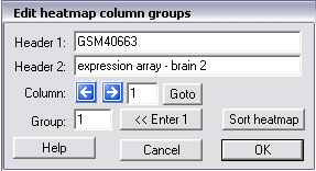
With this command the text shown in the upper row of the "heatmap data" dialogue box may be edited. You can also modify the group number associated with each column of data. Pushing the "Sort heatmap" button will then reorganise the columns in the heatmap such that group numbers appear in increasing order. Change columns with the left and right arrows or use the goto button. To change the group number, enter a number in the "Group" edit box![]() and then push one of the arrows. The contents of the next row will be shown including its group number. In order to speed up editing, the button that is labelled here "<< Enter 1", but that will show "<< Enter n", where n is the previous number entered in the "Group" edit box may be pushed. It is a shortcut that is identical to entering n in the "Group" edit box followed by pushing the right arrow key.
and then push one of the arrows. The contents of the next row will be shown including its group number. In order to speed up editing, the button that is labelled here "<< Enter 1", but that will show "<< Enter n", where n is the previous number entered in the "Group" edit box may be pushed. It is a shortcut that is identical to entering n in the "Group" edit box followed by pushing the right arrow key.
Compare groups
After having defined the experimental groups, in so far this has not already been done by the author of the heatmap, you can visualise (in)significant differences in gene expression levels between these experimental groups. For each heatmap row (gene) Student's test is carried out and a graph as below is created on the current drawing sheet. The expression level of one group is plotted against the expression level of the other. Each dot represents a row and the levels of statistical significance are colour coded as shown in the legend (e.g. gene expression levels on the diagonal, in blue, are to considered to be identical P>0.95).
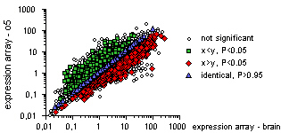
If you select the graph and then choose the pipette tool, the identity of the gene that the pipette points at and the expression levels of the two groups are shown in the status bar:
![]()
The complete result in text format may be obtained if you copy the graph and paste it on Clusters' spreadsheet.

Remove heatmap entries
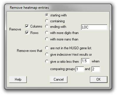
A heatmap may contain entries that seem not to have much meaning or that are not interesting to the user. With this menu item entries answering to certain criteria such as the beginning their gene names can be removed (see the dialogue box below). Genes that are referred to by just a number can be removed using the "with more digits than". Fill in the number of digits in the edit box![]() that contains "LOC" in the figure below. Certain rows or columns may contain too many "not determined" or "Not A Number (nan)" data. Remove those entries using the "with more nans than" option. Again, fill in the number of nans in the "LOC" edit box
that contains "LOC" in the figure below. Certain rows or columns may contain too many "not determined" or "Not A Number (nan)" data. Remove those entries using the "with more nans than" option. Again, fill in the number of nans in the "LOC" edit box![]() .
.
Shorten heatmap
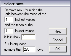
Heatmap data can of course be manipulated on a spreadsheet. For ease of use, several options are also available on the drawing sheet. With the Shorten heatmap command one can remove genes (rows) from the map that are little affected by the experimental conditions. In the dialogue below two ways are proposed to select the genes for which changes with experimental condition are most pronounced. The first option is to remove genes for which the maximum difference in expression within a row is less than a certain factor (2 in the example below). Usually multiple entries for a certain condition exist. In order to prevent the selection of outliers that may be merely the result of experimental error, the critical ratio can be chosen such that is the ratio of the mean of highest expression levels and the mean of the lowest expression levels in a row. In the dialogue box below the means of the 4 highest and lowest levels are taken. The second way to select significant changes is to impose a maximum number of genes (rows) as a result. In the example below a maximum of 285 genes will be retained.
It is advised to apply Shorten heatmap before using the Make cluster or Principal components commands, because genes that are hardly or not affected by the experimental conditions make the calculations more difficult and tend to produce noise in the results.
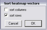
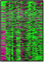
Sort heatmap
The data in the heatmap can be sorted according to differences in expression levels. When sorting rows, the genes for which the expression levels varies the most with experimental condition will end up at the bottom of the heatmap. In the example below the rows in heatmap to the left have been sorted giving the result on the right. Sorting columns goes similarly.
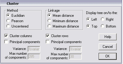
Make cluster (tree)
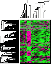
Clustering analysis of a heatmap is carried out with this command. If Clustering has already been carried out on the heatmap in question, then the Cluster dialogue box that pops up shows the parameters that were last used to calculate the clusters. In the example below, the data in heatmap of the last section has been clustered by calculation of the mean Euclidian distance between row vectors and column vectors.
A comprehensive explanation of clustering can be found at the NCBI site. The essentials are reproduced here. Suppose there are n genes, then the Euclidian distance between two out of m (experimental) vectors x and y constituted by n genes is:
Pearson correlation of two vectors of length n, with x-bar is the mean of x and y-bar the mean of vector y is:
The un-centred correlation coefficient of two vectors x an y is:
Before carying the clustering procedure, a column-normalised copy of the data in the heatmap is made. This copy is then used to for the iterative clustering algorithm. In the very beginning there are m clusters containing each a single vector. Next, the two clusters that are closest according to criteria mentioned above are grouped into a new cluster, now containing two members. m-1 clusters remain at that point. Then, the next closest pair of clusters is combined to form a new cluster. Here the "linkage" option becomes important. If the distance of two clusters, each containing multiple vectors is evaluated, it has to be decided what is to be considered as the distance between clusters. In this software three options are proposed. The "Maximum distance" option uses the maximum distance between a vector in cluster 1 with respect to another in cluster 2. The "Minimum distance" option finds the minimum distance between a vector in cluster 1 and the closest in cluster 2. The "Mean distance" option calculates the mean distance between pairs of vectors in the two clusters. The "Maximum distance" option seems the most conservative option. The iterative process is repeated until only one cluster remains.
Vectors creating background noise may be eliminated during the clustering process by using the "Principal Components" (PCs) option. The vectors are first reduced to a length of k < n by Principal Component Analysis (PCA). Then clustering is carried out on the m vectors of length k. Afterwards, the original vectors of length n are sorted accordingly. The number of PCs to use is set with the "Variance" and "Max number of components" options whichever condition is satisfied first. The "Variance" edit box![]() takes a value between 0 and 100% of the total variance to be accounted for by the first k PCs. Putting a very low percentage of variance (0-25) gives bad results, 80-95% is more reasonable (see also the next Principal Components section).
takes a value between 0 and 100% of the total variance to be accounted for by the first k PCs. Putting a very low percentage of variance (0-25) gives bad results, 80-95% is more reasonable (see also the next Principal Components section).
Remove row tree
Removes the row cluster tree beside the selected heatmap.
Remove column tree
Removes the column cluster tree beside the selected heatmap.
Principal components
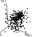
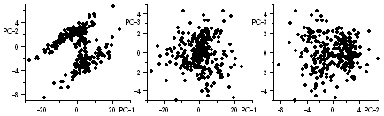
Principal component analysis (PCA) is carried out on a heatmap using this menu item. The three principal components of heatmap below left is show to the right of it. Plotting these three components in 3D space gives the 3rd figure from the left.
The three rightmost graphs represent projections. Two populations of genes appear to emerge in the plot of PC-2 vs PC-1.
3 PC graph
With this menu item a 3D graph representing the three principal column components (PCs) is created directly without creation of a 3 PC heatmap as in the section above. Use the pipette tool to have the gene names corresponding to each dot in the graph shown in the status bar at the bottom of the program's window.
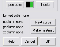
In order to separate two clouds of data in the graph and to create two new (sub-) heatmaps, rotate the 3D graph until the two populations seem well distinct. Then split the 3D graph as explained in the Tools>Split graph section. Next double-click on the 3D graph, push the "Make heatmap" button" in the "3D curve" dialogue box that pops up (see illustration just below), push the "Next curve" button and finally push the "Make heatmap" button" again followed by "OK". Two new heatmaps have appeared on the drawing sheet.
Search the manual: